Exploring the Pacific Arctic Seasonal Ice Zone With Saildrone USVs
 Andrew M. Chiodi1,2*
  Chidong Zhang2
  Edward D. Cokelet2
  Qiong Yang1,2† Calvin W. Mordy1,2
  Chelle L. Gentemann3,4
  Jessica N. Cross2
  Noah Lawrence-Slavas2
  Christian Meinig2
  Michael Steele5 Don E. Harrison2 Phyllis J. Stabeno2
  Heather M. Tabisola1,2
  Dongxiao Zhang1,2
  Eugene F. Burger2
  Kevin M. O’Brien1,2 Muyin Wang1,2
- 1Cooperative Institute for Climate, Ocean and Ecosystem Studies, University of Washington, Seattle, WA, United States
- 2Pacific Marine Environmental Laboratory, National Oceanic and Atmospheric Administration, Seattle, WA, United States
- 3Farallon Institute, Petaluma, CA, United States
- 4Earth and Space Research, Seattle, WA, United States
- 5Polar Science Center, Applied Physics Laboratory, University of Washington, Seattle, WA, United States
More high-quality, in situ observations of essential marine variables are needed over the seasonal ice zone to better understand Arctic (or Antarctic) weather, climate, and ecosystems. To better assess the potential for arrays of uncrewed surface vehicles (USVs) to provide such observations, five wind-driven and solar-powered saildrones were sailed into the Chukchi and Beaufort Seas following the 2019 seasonal retreat of sea ice. They were equipped to observe the surface oceanic and atmospheric variables required to estimate air-sea fluxes of heat, momentum and carbon dioxide. Some of these variables were made available to weather forecast centers in real time. Our objective here is to analyze the effectiveness of existing remote ice navigation products and highlight the challenges and opportunities for improving remote ice navigation strategies with USVs. We examine the sources of navigational sea-ice distribution information based on post-mission tabulation of the sea-ice conditions encountered by the vehicles. The satellite-based ice-concentration analyses consulted during the mission exhibited large disagreements when the sea ice was retreating fastest (e.g., the 10% concentration contours differed between analyses by up to ∼175 km). Attempts to use saildrone observations to detect the ice edge revealed that in situ temperature and salinity measurements varied sufficiently in ice bands and open water that it is difficult to use these variables alone as a reliable ice-edge indicator. Devising robust strategies for remote ice zone navigation may depend on developing the capability to recognize sea ice and initiate navigational maneuvers with cameras and processing capability onboard the vehicles.
Introduction
The spring/summertime retreat of Arctic sea ice exposes approximately 107 km2 of the ocean surface to direct exchanges of heat, momentum and carbon dioxide (CO2) with the atmosphere in an area referred to as the seasonal ice zone (SIZ; Steele and Ermold, 2015). Knowledge of these fluxes is necessary to understand Arctic weather, climate, and ecosystems (Danielson et al., 2020; Lu et al., 2020; Ouyang et al., 2020; Qi et al., 2020; Terhaar et al., 2020). Accurate knowledge of the fluxes and the surface variables from which they are estimated, such as sea surface temperature (SST), surface pressure, humidity, air temperature, and wind speed and the partial pressure of carbon dioxide (pCO2) is useful for a variety of applications, including accurate initialization and validation of numerical weather forecast models (Liu et al., 2015; Zhang et al., submitted).
Since satellite-based estimates of sea-ice extent became routinely available in the late 1970s, summertime minimum (September) Arctic ice extent has noticeably declined (Wang and Overland, 2009, 2012; Stabeno and Bell, 2019), the ice season has shortened (Wang et al., 2018; Stabeno, 2019) and Arctic surface temperatures have risen faster than global mean surface temperatures (Serreze and Francis, 2006; Danielson et al., 2020). Results from climate forecast model experiments have projected that Arctic surface temperatures will continue to rise significantly faster than the global mean (Alexander et al., 2018), partly as a result of the coupling between diminishing Arctic sea ice and its effects on the surface to atmosphere heat flux (Walsh, 2014; Kashiwase et al., 2017). Accurate knowledge of surface heat and momentum fluxes and how they change with varying sea-ice concentration is necessary for further development and verification of Earth system models.
Few high-quality, direct measurements of surface oceanic and atmospheric variables are available in the Arctic SIZ. The benefits of using automated, uncrewed sampling platforms to increase our ability to observe the SIZ has been demonstrated by several research programs (see Lee et al., 2017, and references therein). Recent SIZ sampling strategies include deploying instrumentation on or in the ice (e.g., Polashenski et al., 2011; Timmermans et al., 2014; Gallaher et al., 2017), or on autonomous underwater vehicles and open water platforms, such as moored-buoys and wave gliders (Wood et al., 2013). Surface drifters (e.g., Thomson, 2012; Banzon et al., 2020) capable of measuring environmental parameters such as air and water temperature and wind speed, have also been deployed in open water and partial ice cover. Uncrewed surface vehicles (USVs) that can navigate from open water through ice zones, while collecting the observations needed to estimate (Bourassa et al., 2013) surface fluxes, would add a key component to our existing high-latitude observing capability. In summer 2019, a collaboration between NOAA, University of Washington and NASA investigators led to the deployment of five USVs, saildrones, with the objective of collecting such observations and providing a subset of them to forecast centers in real time. Saildrones are wind-driven, solar-powered and outfitted for this mission to measure near-surface wind speed and direction, humidity, air temperature and barometric pressure, upper ocean currents, SST, sea surface salinity (SSS), downward longwave and shortwave radiation, and pCO2, among other variables (Cokelet et al., 2015; Meinig et al., 2015; Mordy et al., 2017; Zhang et al., 2019). A main mission objective was to measure these quantities in the SIZ up to the ice edge. Other objectives of the mission included collecting in situ observations for improving calibration of satellite-based measurements of SST in polar waters, occupying four Distributed Biological Observatory lines (Grebmeier et al., 2019), performing pCO2 sensor cross-calibration tests with instrumentation aboard the USCGC Healy, ocean current surveys of Hanna Shoal, the Chukchi Shelf Current and the Alaskan Coastal Current (c.f. Li et al., 2019) and collecting data for surface flux estimates over Chukchi Sea regions being sampled simultaneously by Air Launched Autonomous Micro-Observer (ALAMO) profiling floats (Jayne and Bogue, 2017) and Beaufort Sea regions being sampled simultaneously by Seagliders (Eriksen et al., 2001) deployed during the Stratified Ocean Dynamics in the Arctic (SODA) experiment (Lee et al., 2016).
The saildrones were launched from Unalaska, AK, United States, in early May 2019, and sailed northward through Bering Strait in early June 2019. In order to successfully complete the mission, they would need to navigate through the SIZ and return to Unalaska before the combination of the energy stored in the vehicle’s batteries and availability of solar power diminished below levels necessary to sustain vital communication, navigation and sensor functionality. Navigational information such as vehicle speed over ground and heading was relayed to the navigational team, with typically a few to several minutes delay. Four cameras mounted on the wing also provided images, which took ∼30 min to be transmitted. These photos provided three perspectives: (i) upward-looking views of the sky; (ii) downward views of the vehicle hull and surrounding environs (e.g., Figure 1A); and (iii) horizontal views fore and aft of the wing (e.g., Figure 1B). The downward-looking photos in particular provided clear confirmation of times when the vehicles were in contact with or immediately next to sea ice.
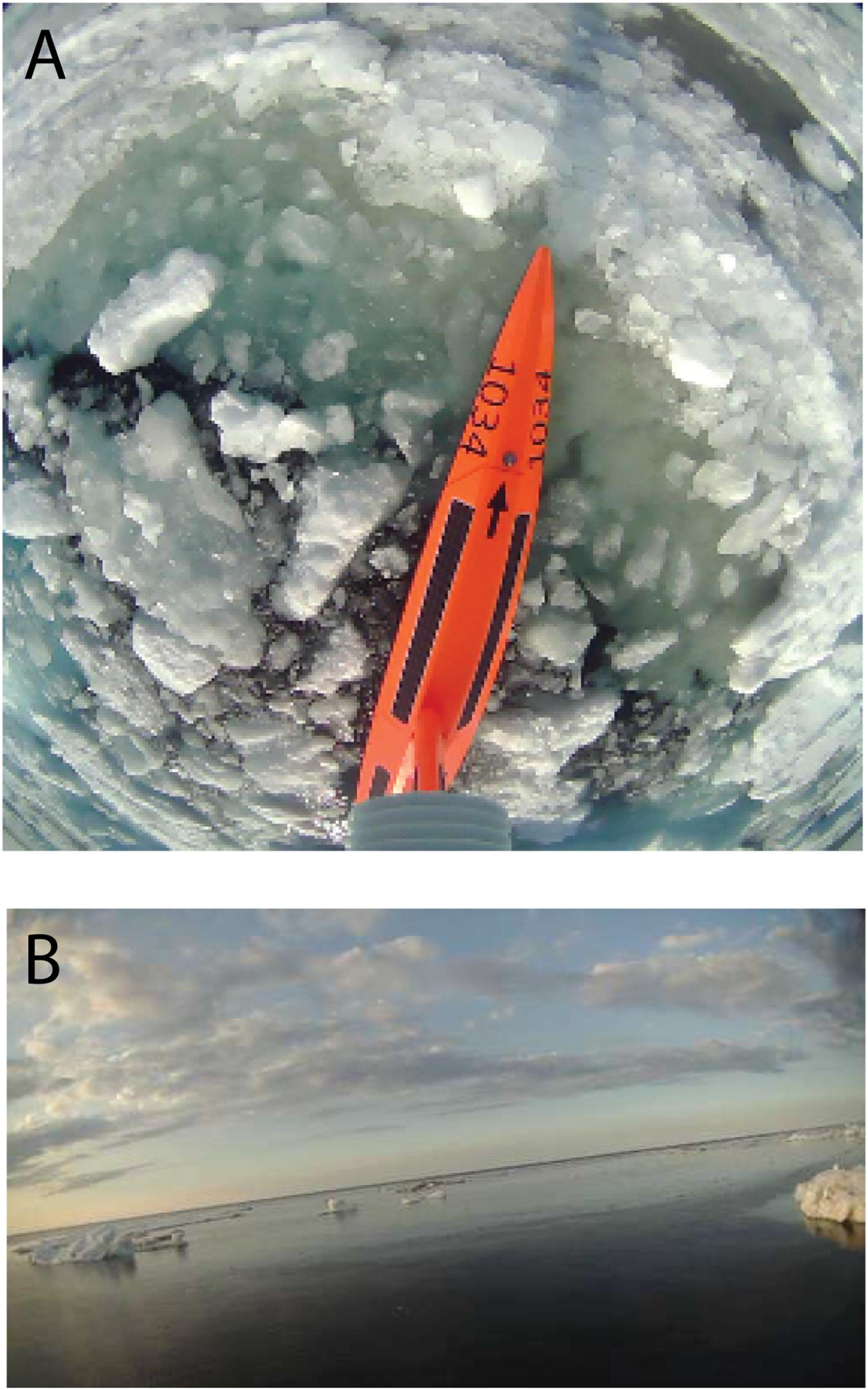
Figure 1. Examples of (A) downward-looking image taken atop the saildrone wing while in sea ice, and (B) horizontal image from the saildrone wing with sea ice floes visible.
Modern ice-navigation strategies for ships (e.g., Stoddard et al., 2016; Transport Canada, 2018) pair information about ship structure and capability (e.g., IACS, 2016) with estimates of ice concentration and type to assess risks along a route. Navigation-relevant ice information is available from a variety of sources offering different spatial resolutions and collection intervals (e.g., Hui et al., 2017; Rainville et al., 2020). Satellite information available presently includes passive microwave estimates of ice concentration, optical imagery and synthetic aperture radar (SAR) imagery. SAR offers the advantages of all-weather capability and relatively high spatial resolution compared to passive microwave data (e.g., Zakhvatkina et al., 2017 evaluate ice-water classification from Radarsat-2 ScanSAR images with 50 m × 50 m pixel spacing; see also Bertoia et al., 2004; Hui et al., 2017). The general use of individual wide-swath and relatively high-resolution SAR images, however, is limited by the large proportion of them that are not publicly available (Zakhvatkina et al., 2019). Several national ice centers synthesize ice distribution information from multiple sources and expert analysis to produce weekly to bi-weekly ice charts for strategic planning. The “tactical,” or most direct navigational utility of ice-distribution information is usually limited to <24 h from the time it was collected (Scheuchl et al., 2004; Rainville et al., 2020).
The suite of remotely produced ice information potentially available for a USV mission such as ours is basically the same as for ships. The questions asked of the ice information, however, may be somewhat different in each case. For example, Canadian Arctic experience has shown that sufficiently powered, ice-strengthened ships can make progress through first-year ice in concentrations up to 7/10ths without assistance from an icebreaker (Ice Navigation in Canadian Waters, 2012). Thus, navigating a Polar Class 6 or 7 ship (IACS, 2016) requires, particularly, information about where the ice distribution exceeds these criteria (c.f. Smith and Stephensen, 2013). Saildrones are not specifically designed to withstand collision with or push through sea ice, substantially limiting the range of ice conditions safely navigable compared to ice-strengthened ships. Most ships should also be able to “steer at slow speed around the floes in open pack ice [<6/10ths ice] without coming into contact with very many of them” (Ice Navigation in Canadian Waters, 2012). The capability to steer through floes is perhaps what most clearly distinguishes ship navigation from the situation faced by the USVs on our mission.
Saildrones navigate primarily by controlling the angle of the rudder and the vertically oriented, rigid wing, which functions in roughly the manner of a mainsail on a traditional sailboat. They automatically navigate from waypoint to waypoint, accounting for wind and currents, while remaining within a specified corridor. The waypoints were decided by scientists and uploaded to the vehicles by Saildrone, Inc. pilots. The saildrones were not equipped during this mission with an automated capability to avoid collision; if their uploaded route intersected a floe, the vehicles would contact the floe unless re-routed by the pilot. In order for the objectives of this mission to be accomplished, the vehicles needed to repeatedly navigate in close proximity to sea ice. Several different types of information were considered or referred to during the mission to help with this navigational challenge. These sources included daily gridded satellite estimates of sea-ice concentration over the study region, natural color (optical) images of the surface provided by satellite radiometric measurements, SAR imagery and the daily 10% sea-ice concentration contour produced via multisensor analysis at the US National Ice Center (NIC). Information collected aboard the vehicles such as near-surface ocean temperature and salinity and the images from the vehicles’ wings were also used.
The vehicle images and navigational metrics such as speed-over-ground provide a de facto record of when the vehicles were embedded in or in close proximity to ice floes. Here, we examine the relationships between this de facto record and the other (potential) sources of sea-ice distribution information that were considered or used while remotely navigating these five saildrones through the SIZ of the Chukchi and Beaufort Seas during May–October 2019. Our focus here is on products available publicly at daily, or higher, frequency and the observations and images collected by the USVs. Our objective in this article is to highlight both the challenges and strategies for improving remote ice navigation with USVs. Results may thereby provide a step forward for our wider objectives of understanding what sort of USV array is needed to monitor the Arctic (or Antarctic) SIZ in support of initializing and assessing the skill of operational numerical weather prediction systems and climate models, and validating numerical and satellite estimates of Arctic surface fluxes.
Materials and Methods
In situ Observations
The saildrones deployed on this mission were part of a collaboration between Saildrone, Inc.1 and the National Oceanographic and Atmospheric Administration (NOAA) Pacific Marine Environmental Laboratory (PMEL; Meinig et al., 2019) through a Cooperative Research and Development Agreement. Saildrones have ∼ 7 m long hulls, rigid-wing heights 5 m above the water line, and keel depths of 2.5 m. The saildrone routes were coordinated with members of Alaska’s North Slope and Northwest Arctic Boroughs and communicated through the United States Coast Guard Notice to Mariners to avoid potential interference with other uses of the Alaskan waterways. The vehicles’ progress was monitored remotely by scientific and engineering team members. Batteries and solar panels power the onboard navigational electronics, which included automated identification system transceivers and Global Positioning System (GPS) navigational systems, as well as scientific instrumentation and satellite telemetry of data and navigational instructions. We designated the five saildrones deployed on this mission sd-1033, sd-1034, sd-1035, sd-1036, and sd-1037. Each was equipped with the following sensors: a Rototronic HC2-S3 sensor at 2.3 m height measured air temperature and relative humidity; a Sea-Bird SBE37 Microcat at 0.5 m depth measured seawater conductivity and temperature, which together provide seawater salinity; a Vaisala PTB210 Barometer on the hull (0.2 m height) measured sea level pressure; and a Gill model 1590-PK-020 anemometer atop the wing (5.2 m height) provided three dimensional wind velocity at 10 Hz. These wind measurements, along with synchronous measurements from the onboard inertial measurement unit (VectorNav model VN-300) and GPS, allowed for geo-referenced wind velocity to be calculated onboard and telemetered to the Global Telecommunications System and onshore data repositories as 1-min averages (as described in more detail in Zhang et al., 2019). The higher frequency data were stored onboard for access upon vehicle recovery. Zhang et al. (2019) reported that the auto-corrected saildrone wind speeds measured as a part of the Tropical Pacific Observing System – 2020 pilot study had RMS differences of 0.6 m s–1 with respect to the benchmark observations collected on the Salinity Processes in the Upper ocean Regional Study 2 (SPURS-2) buoy. This was based on hourly averages collected while the saildrones were within 12 km of the buoy, during which time the buoy measured a mean speed of 4.2 m s–1, standard deviation of 1.9 m s–1 and maximum (minimum) wind speed of ∼9.2 (0.2) m s–1. A saildrone’s speed over ground is dependent upon wind velocity, ocean current velocity, and navigation. Over the course of this Arctic mission, the vehicles measured an average wind speed of 5.4 m s–1, and their average speed, with respect to the Earth’s surface, excluding the times in which they were embedded in or left to drift with sea ice, was 0.96 m s–1, or ∼18% of wind speed. The maximum hourly averaged vehicle speed recorded during this mission was 2.9 m s–1 at an hourly mean wind speed of 12 m s–1 (sd-1035 on 19 July 2019). Sd-1033 and sd-1034 were equipped with Autonomous Surface Vehicle CO2 (ASVCO2; Sutton et al., 2014; Sabine et al., 2020) sensors capable of measuring pCO2 in both the air and water. Along with wind speed, this pCO2 information provided the basis for estimating the air-sea flux of carbon dioxide. ASVCO2 systems have been described and evaluated previously by Sabine et al. (2020) and found to provide pCO2 observations within ±2 μatm of shipboard systems and moored autonomous pCO2 systems. Sd-1033 and sd-1034 also had instruments capable of measuring solar irradiance, longwave radiation, ocean skin temperature (experimental), ocean color (Chl-a, CDOM), dissolved oxygen, pH and ocean current speed and direction (acoustic Doppler current profilers).
All of these saildrones, except sd-1037, were deployed with cameras mounted on their wings that provided three perspectives: (i) upward-looking views of the sky; (ii) downward views of the vehicle hull and surrounding environs (e.g., Figure 1A); and (iii) horizontal views fore and aft of the wing (e.g., Figure 1B). The saildrones sent back images every 5 to 60 min over most of the mission, but cameras were turned off during later stages of the mission to conserve power. The cameras on sd-1035 and sd-1036 collected images at a resolution of 1920 × 1080 pixels. The camera on sd-1034 was lower resolution (500 × 279).
The Saildrone-derived data used in this paper are hosted at PMEL by its Science Data Integration Group. These data are received from Saildrone during the mission and also as a bulk data acceptance post-mission. Data were delivered from Saildrone as discrete sampling geometry NetCDF files that included comprehensive documentation of the observations, including the standard and long names of the observed variables, their units, latitude, longitude and time of collection, as well as the name, vendor, serial number, installation height on the vehicle, installation date, date of last calibration, and sampling schedule of the sensor, among other information. During the mission, data files containing 1 min observations were delivered twice per hour, while high resolution (10 Hz and 1 Hz) data were delivered post-mission.
A subset of the 1-min observations received in near-real time were disseminated on the World Meteorological Organization (WMO) Global Telecommunication Service (GTS). The GTS is an operational network maintained by the WMO for the near-real time dissemination of environmental observations to be used in operational forecasting by global weather services. From this mission, an observation every 10 min was uploaded onto the GTS using the Global Ocean Observing System Observations Coordination Group developed Open Access to GTS framework, in partnership with PMEL and the NOAA National Data Buoy Center. This framework was developed to ease the process of globally distributing data in near-real time on the GTS for data producers such as Saildrone, Inc.
A saildrone (sd-1023) on a previous hydroacoustic survey in the Chukchi Sea (Levine et al., 2020) had a brief encounter with sea ice on 7 August 2018 at 71.5°N, 162°W. We analyzed its position, measurements and photographs with regard to various sea-ice products to obtain a preliminary evaluation of what information might be useful for guiding saildrones in sea ice.
To facilitate comparison between the in situ saildrone conditions and other potential sources of sea ice information, we define two in situ sea ice-related quantities. The first is called the “In Situ Sea Ice (ISSI)” record and is defined as 1 over the periods during which ice was visible in the downward or horizontal saildrone images and 0 when ice was not visible in the saildrone images. We use the term “ice free” in reference to the saildrone images. The resulting time series facilitates examination of the distributions of SST, salinity, and other observations collected while ice was or was not visible in the saildrone images. The second quantity is called “Ice-Blocked Vehicle (IBV)” and keys on the points at which the saildrones were blocked by ice on transects beginning in ice free water. Blockage points were determined based on un-commanded drops in vehicle speed-over-ground and inspection of saildrone images (discussed in more detail in the “Results” section). Knowing these ice-blockage points allows us to tabulate information about the changes in SST and salinity observed while approaching ice floes from open water. We use 3 h as the approach period based on preliminary examination showing that 3 h is long enough to capture some ice-free observations and the maximum negative SST and temperature gradients observed en route to the ice, yet short enough that ice-free measurements do not overly dominate the analysis and the vehicle route segments prior to IBVs did not, typically, include substantial changes in direction (e.g., change in USV heading of ∼180°).
Satellite Information
The European organization for the exploitation of satellite measurements (EUMETSAT) offers daily gridded sea-ice concentration estimates based on radiances measured by the satellite-born Advanced Scanning Microwave Radiometer (AMSR-2). Hereafter, we refer to EUMETSAT’s daily AMSR-2 ice concentration product as EA2. EA2 daily estimates are available starting in September 2016 on a 10 km horizontal resolution polar stereographic grid. Daily EA2 updates were typically available to us in the early local morning hours (Pacific Daylight Time = Universal Coordinated Time – 7 h) and were considered for use in route planning during the mission. The relationship between the EA2 values interpolated to the vehicles’ positions and the in situ conditions encountered by the vehicles is further examined herein. To facilitate this examination, interpolated EA2 estimates have been binned at 1% concentration intervals with the first bin (labeled 0%) containing all 0% concentration estimates, the second, 1%, containing concentrations >0% and ≤1%, the third, 2%, containing concentrations >1% and ≤2%, and so forth. Herein, we calculate the ice extent of our study region as the area of EA2 grid cells within the region bounded by 145°W–180°W and 66°N–80°N with >10% ice concentration, in keeping with the definition used by the NIC. Lavelle et al. (2016) evaluated EA2 concentrations in reference to weekly ice charts produced by the NIC. This comparison was done on a grid point-by-grid point basis and found that the spatially aggregated percentage of Northern Hemisphere grid points with concentrations within 10% of one another was between 90 and 95% during their 1 January – 31 December 2015 analysis period, with the exception of mid-June through August when this percentage fell below 90% and reached a minimum of ∼83% in mid-July. Lavelle et al. (2016) suggest summertime melt caused this drop in weekly ice-chart versus EA2 concentration agreement (c.f. Markus and Dokken, 2002).
A daily analysis of sea-ice information, based on multiple sources of near real-time satellite data, derived satellite products, buoy data, and other weather data was provided to us upon request by the NIC. A main component of this analysis was its ice edge, which is nominally defined as the 10% sea-ice concentration contour. The NIC 10% concentration contour is produced by NIC analysts with the aid of several types of satellite imagery, including Advanced Very High Resolution Radiometer, Special Sensor Microwave Imager, Moderate Resolution Imaging Spectroradiometer (MODIS), Visible Infrared Imaging Radiometer Suite (VIIRS) and SAR (e.g., Lavelle et al., 2016). The latitude and longitude points comprising the daily NIC ice-edge contour are freely available to the public (U.S. National Ice Center, 2020). The NIC ice edge was consulted during mission days with an ice-navigation component, which included the majority of days when at least one vehicle was north of Bering Strait (5 June 2019 – 28 September 2019).
We occasionally requested extended analysis from NIC when the Radarsat-2 SAR images available to them (c.f. Bertoia et al., 2004) covered the saildrone positions. Radarsat-2 return periods from <1 to 3 days are typical for Chukchi and Beaufort Sea locations [interested readers can freely view reduced-resolution Radarsat-2 images on the European Space Agency Earth Observation Portal2 as well as the SODA situational awareness data archive3 (Rainville et al., 2020)]. High-resolution Radarsat-2 imagery, however, is not freely available to the public. The enhanced assistance received from NIC confirmed that the ability to geo-locate USVs on full-resolution SAR imagery within the tactical window (Scheuchl et al., 2004 suggests this to be <6 h) is a critical tool for remote ice navigation.
Satellite imagery from the European Space Agency Sentinel-1 SAR and Sentinel-2 MultiSpectral Instrument (MSI) missions is made freely available from the Sentinel Hub EO Browser4 and was used during the mission. Sentinel-2 consists of a pair of satellites with MSIs measuring 13 spectral bands in the 443–2203 nm range with 10–60 m horizontal resolution (König et al., 2019). The return period for Sentinel-2 MSI images in the Chukchi and Beaufort Seas was up to 1 per day. Use of MSI imagery for ice detection, however, requires clear sky conditions. Sentinel-1 SAR provides all-weather capability (e.g., Nagler et al., 2015; Karvonen, 2017). Based on the EO Browser repository, however, the Sentinel-1 return period for a specific location in our study area was up to 12 days.
The natural color images made available at the NASA Worldview website5, offered useful information about ice distribution, provided the local cloud cover was sufficiently sparse. Images are available on a daily basis from this site based on measurements collected by pairs of VIIRS and MODIS instruments aboard four different satellites, with a different image layer for each combination and a nominal horizontal resolution of 250 m. Because the cloud patterns tended to shift more than the ice between the different satellite overpasses during a given day, having multiple sensor-layers (e.g., the MODIS image from the Aqua v. Terra satellite) was sometimes useful for distinguishing sea ice from cloud.
Results
Daily Gridded Sea-Ice Concentration From AMSR Measurements
Illustrations of the EA2 gridded sea-ice concentration estimates are shown in Figures 2, 3 on the days of the first and final ice encounter (ISSI and IBV) of the mission, i.e., 14 June 2019 and 23 August 2019, respectively. In these two cases, saildrones encountered sea ice near the NIC 10% concentration lines; however, other ice encounters occurred in a wide range of sea-ice concentrations.
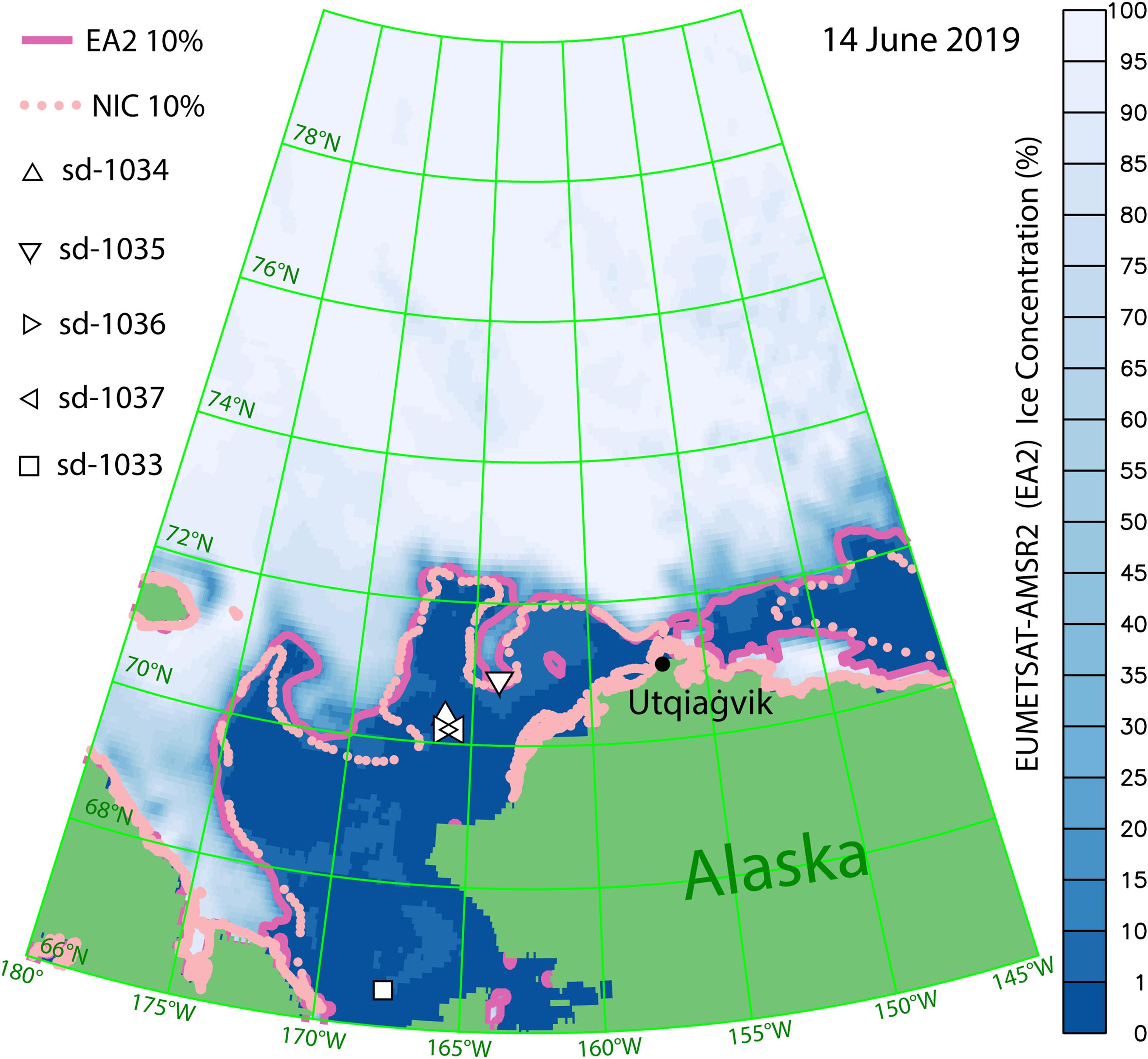
Figure 2. The Eumetsat-AMSR2 (EA2) estimate of sea-ice concentration (blue-white hues) and 10% ice contour (solid purple curve) along with the NIC ‘ice edge’ 10% contour (pink dotted curve) and locations of saildrones sd-1033 (square), sd-1034, sd-1035, sd-1036, and sd-1037 (triangles) on 14 June 2019, the date of the mission’s first ice encounter (sd-1035).
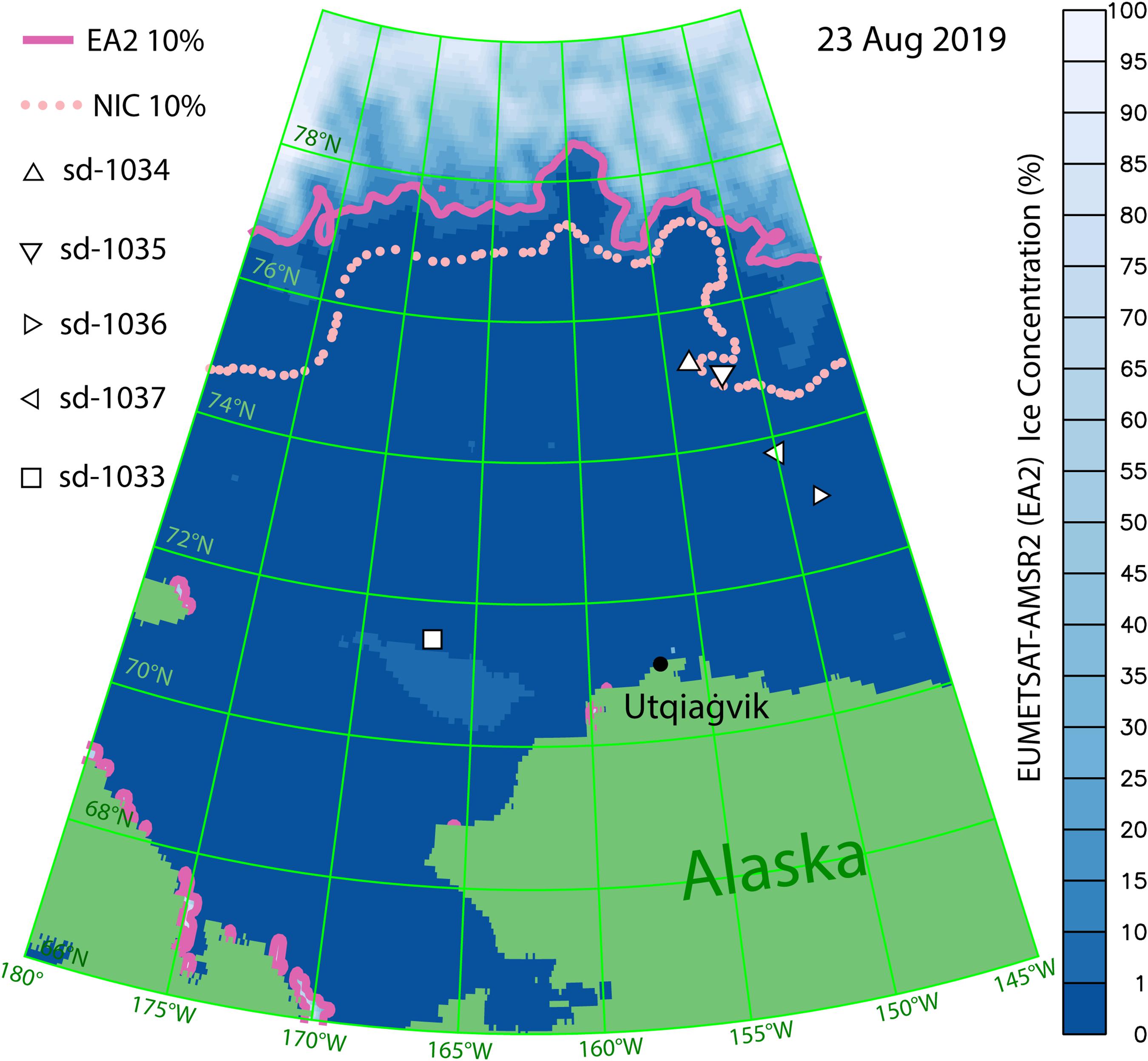
Figure 3. The Eumetsat-AMSR2 (EA2) estimate of ice concentration (blue-white hues) and 10% ice contour (solid purple curve) along with the NIC ‘ice edge’ 10% contour (pink dotted curve) and locations of saildrones sd-1033 (square), sd-1034, sd-1035, sd-1036, and sd-1037 (triangles) on 23 August 2019, the date of the mission’s last ice encounter (sd-1035).
Based on EA2, ice extent over the study region bounded by 180°–145°W and 66°N–80°N was ∼10 × 105 km2 at the start of the mission on 15 May 2019 (Figure 4). The vehicles encountered ice during different phases of the ice retreat over this region. A moderately paced decline of −0.92 × 10⁵ km2/month was observed in June 2019 based on a linear fit to the EA2 concentration estimates. A more rapid decline was seen in July and early August (−3.8 × 10⁵ km2/month). The pace of the decline in regional ice extent then slowed in mid to late August, during which time ice extent hovered near 2 × 10⁵ km2. The study area minimum ice extent of 1.28 × 10⁵ km2 occurred on 15 September 2019. Comparison reveals that the study region experienced an earlier decline in ice cover in 2019 relative to the previous two summers over which EA2 data are available (Figure 4). On 28 July 2019, study-region ice extent reached 5 × 10⁵ km2, a level not reached until 2 August in 2017 and 16 August in 2018. The return of ice to the study region in 2019 was also slower than in the previous 2 years: In 2017 and 2018 ice extent had risen to 5.6 and 6.2 × 10⁵ km2, respectively, by the end of October but was still at 2.4 × 10⁵ km2 at the end of October 2019, based on EA2.
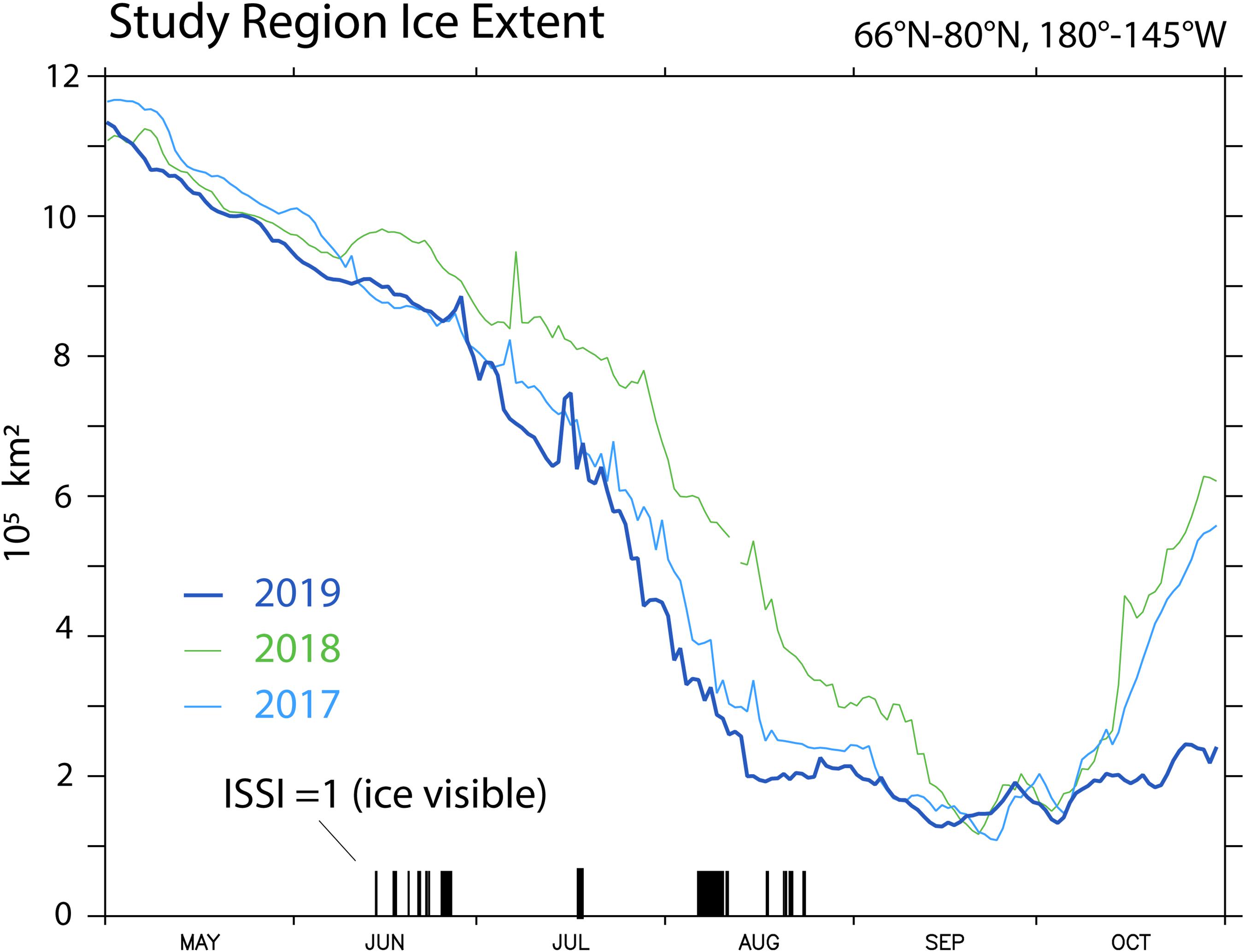
Figure 4. Sea ice extent over the Chukchi and Beaufort Sea study region (180°–145°W, 66°–80°N) from the AMSR2 based ice concentration estimate provided by the EUMETSAT ocean and sea ice satellite application facility. Vertical lines on the time axis mark times when ISSI = 1, that is, sea ice was visible in either the horizontal or downward saildrone images. ISSI = 0 (images were ice-free) during all other times, which are not marked by vertical lines.
The distribution of EA2 sea-ice concentration at the locations of sd-1034, sd-1035 and sd-1036 is shown in Figure 5. Based on EA2, these three vehicles collected observations in sea-ice concentrations from 0 to slightly over 20%. The most common EA2 estimate was for 0% concentration at the vehicles’ locations (59%). Three percent of the observations have an EA2 estimate of 10% concentration or greater. A secondary maximum occurs at ∼16% sea-ice concentration.
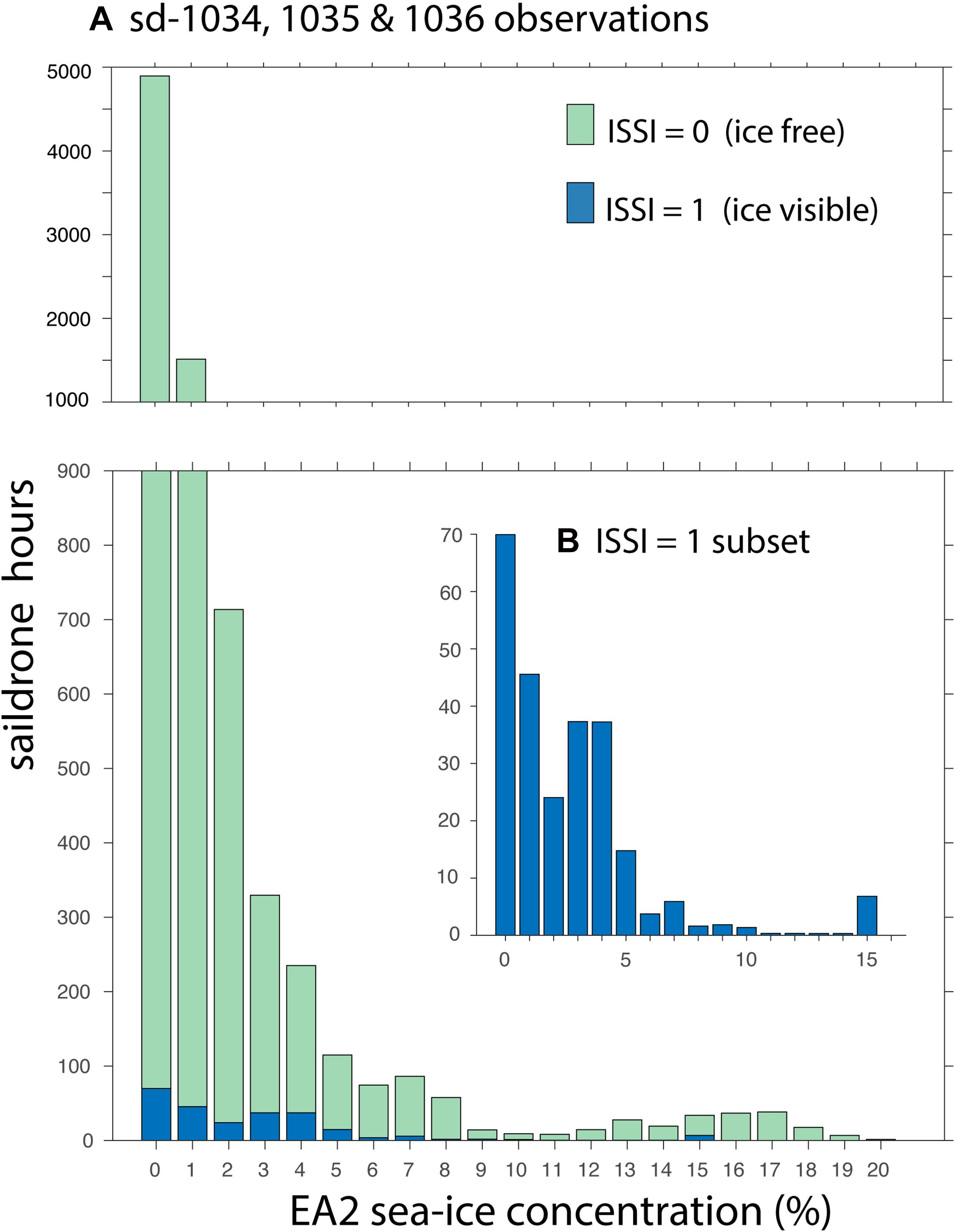
Figure 5. (A) Histogram showing the number of hours saildrones spent in different EA2 sea-ice concentration levels. Data are from sd-1034, sd-1035, and sd-1036 and binned in 1% intervals over the period 5 June 2019 – 30 September 2019. (B) The inset histogram highlights the subset of observations collected when ISSI = 1, meaning sea ice was visible in the images taken from the saildrones.
For the subset of observations taken while sea ice was visible in the saildrone images, the most common EA2 estimate at the vehicle locations was still 0% sea-ice concentration. A secondary maximum spans 3% and 4% ice concentration, each with ∼36 h of saildrone observations (inset of Figure 5). There were 8.3 h of observations collected with sea ice visible in the saildrone images and an EA2 estimate of 15% sea-ice concentration. The saildrones encountered ice 1.5% of the time their EA2 concentrations were 0%, 5.8% of the time their EA2 concentrations were 1–10% and 4.1% of the total time they spent in EA2 concentrations >10%, although no sea ice was evident in the vehicle images when the EA2 estimates were >15%.
Ice Edge Information From the U.S. National Ice Center
The EA2 and NIC 10% contours did not always agree, as for example shown in Figures 2, 3. We quantified the uncertainty between these two estimates of the 10% sea-ice concentration edge by calculating the minimum distance between each point on the NIC contour and any point on the EA2 contour, as well as calculating the minimum distance between each point on the EA2 contour and any point on the NIC contour. This calculation was performed in both directions because the ice edge geometry was often sufficiently complex that doing it in only one direction led to an incomplete estimate of distance. We did this for all points on the 10% contours within our study region (Figures 2, 3) and over water; but not along the coast. The results of averaging these contour-separation distances over each day of the mission (Figure 6) reveal that mean minimum-separation distances varied by almost a factor of 20 during the mission, with lows of ∼ 10 km in early June, late September and early October and highs near 175 km in August. The mean minimum distance between the EA2 and NIC 10% ice contours was greatest when the sea-ice coverage was declining rapidly (early to mid-August) and hovering (late-August) approximately 50% above the eventual minimum (c.f. Figures 4, 6). Because the NIC 10% contour may be overestimating the extent of ice (see U.S. National Ice Center, 2020, p. 9 and Figure 7) we looked for better EA2 versus NIC agreement using 8% and 5% contours from EA2. The Figure 6 results, however, remained qualitatively and quantitatively similar using these lower concentration EA2 contours. For example, the minimum, maximum and mean of Line C in Figure 6 changed by ≤7% (see Supplementary Figure 1).
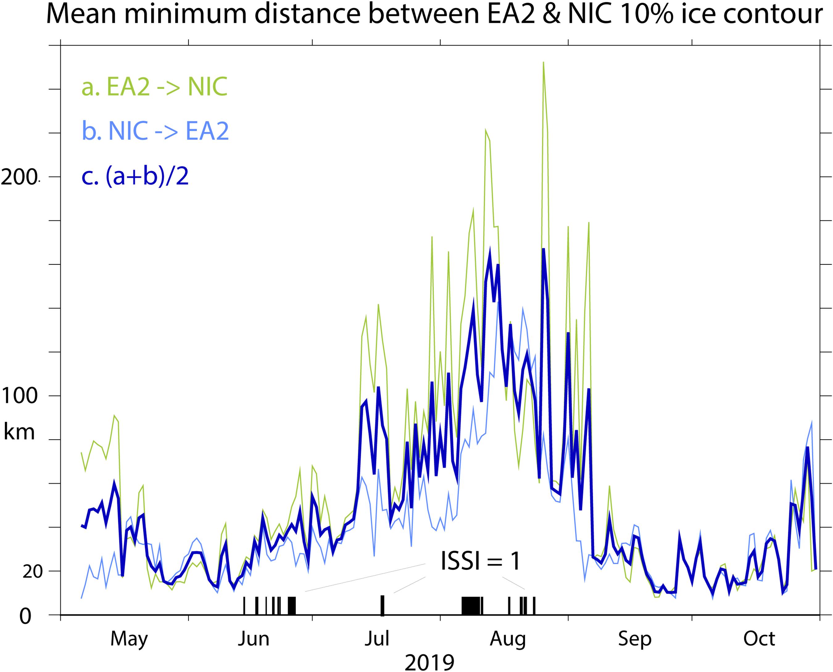
Figure 6. Mean minimum-distances between the 10% ice concentration contour based on the NIC analysis and EA2 data. Vertical lines on the time axis mark times when ISSI = 1. ISSI = 0 during times unmarked by such vertical lines.
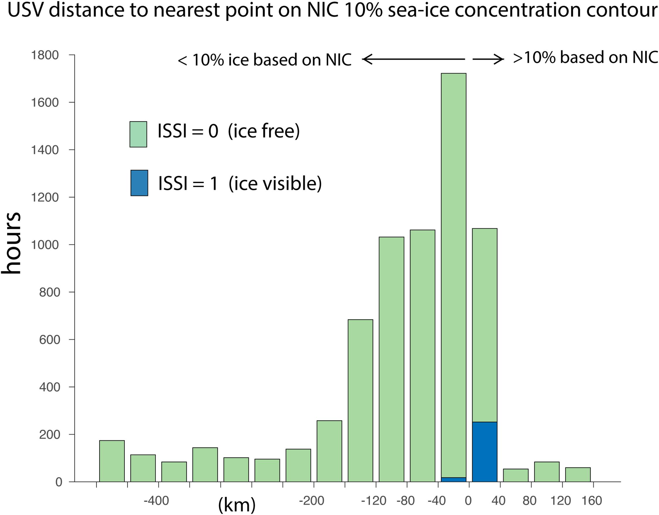
Figure 7. Histogram showing the number of hours that saildrones with cameras (sd-1034, sd-1035, and sd-1036) spent at various distances to the NIC 10% sea-ice concentration contour. Results shown were calculated based on 6-h intervals over the period bounded by their northward transit of Bering Strait on 5 June 2019 through the end of September. The portion of the distribution with sea ice visible from the onboard horizontal or downward photos (ISSI = 1) is shown in blue.
Figure 7 shows the number of hours that the saildrones with cameras (sd-1034, sd-1035, and sd-1036) were within a given distance of the NIC 10% ice edge between 5 June when they entered Bering Strait and the end of September when they turned south. Overall, ∼40% of this time was spent within 40 km of the NIC ice edge; further, 18% of the period was spent in waters with >10% ice concentration according to NIC. Did the saildrone cameras agree with these NIC ice estimates? The answer is mostly yes; nearly all camera images that showed ice were for vehicles in >10% ice concentration according to NIC and ice free conditions were encountered 99.7% of the time the saildrones were in <10% concentration according to NIC. However, 80% of the images taken while the vehicles were in ≥10% ice concentration according to NIC showed no ice. The results confirm that the NIC ice edge corresponds to the boundary beyond which ice may affect vehicle navigation, although the NIC ice edge might be overestimating the extent of ice.
Satellite Imagery
The Terra/MODIS image shown in Figure 8A depicts a zonal ice band that was targeted for exploration on 13 July 2019, with the fleet 130 km to its south. Unfortunately, another clear image did not become available before the fleet contacted sea ice near this location in the first hour (UTC) of 18 July 2019, 5 days later (Figures 8B–F). Thus, waypoints estimated at the ice edge based on the 13 July 2019 image, but used for ice navigation on 18 July 2019, did not account for the distances that the targeted ice band might have moved, dispersed or otherwise changed shape over these 5 days. As it turned out, sd-1034, sd-1036, and sd-1037 encountered sea ice on 18 July 2019 1 to 4 km north of where the southern ice edge was on 13 July 2019.
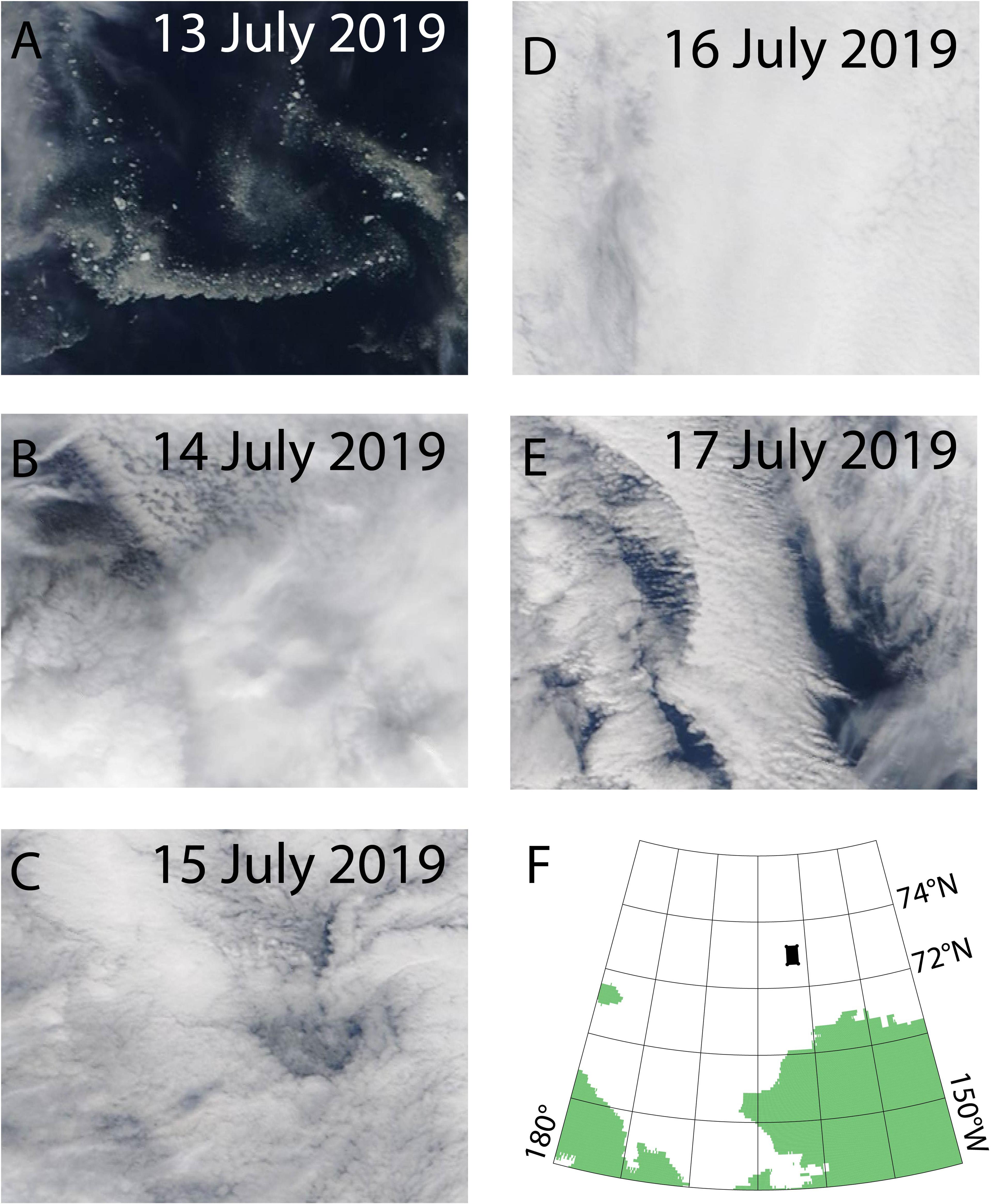
Figure 8. Daily “natural color” images from the MODIS instrument aboard the Terra satellite. These images are centered at 161.46W, 72.97N and span approximately 60 km meridionally (vertical) and 18 km zonally (horizontal). The ice edge visible in panel (A) was targeted for exploration on 13 July 2019, but skies remained cloudy from 14 July through contact with the remnants of the band in the first hour (UTC) of 18 July panels (B–E). The black rectangle in panel (F) shows the location of the images.
Visual inspection of the sequence of daily Terra/MODIS images revealed that mostly clear sky conditions, such as seen in Figure 8A, occurred over this location on about 70% of the days in June 2019, but only about 20% of the days in July 2019 and even fewer days in August. Such unobstructed images of the surface were useful for ice zone navigation when available. However, they could not be consistently relied upon throughout the mission because of cloud cover.
When cloud cover was sufficiently sparse, Sentinel-2 offered relatively high-resolution images (10–60 m), often ∼24 h apart. Example clear-sky images encompassing sd-1034’s route on 18 and 19 June 2019 are offered in Supplementary Figure 2. At the sensing time of the first image (18 June 2019 22:46), sd-1034 was 9 km south of a sparse band of ice extending east from the southern tip of denser pack ice (upper-left corner of Supplementary Figure 2A). By the sensing time of the second image (19 June 2019 23:06), sd-1034 had traveled ∼18 km to the northeast and was ∼1.5 km east of the dense pack ice. In between these two images, sd-1034 became embedded in ice (vehicle images collected at 19:00 UTC confirm ice in the downward view) and then freed itself around 22:15 UTC by sailing east into open water. This episode served as a reminder that the effective navigational resolution of satellite ice imagery is a function of the spatial resolution of the image, the speed of the vehicle, and the distance that the ice moves after the image is available. The ice moved ∼10 km in this case.
A few days prior, at ∼09:00 on 17 June 2019, sd-1036 and sd-1037’s routes intersected an ice floe visible in the Sentinel-2 image collected at 22:56 on 16 June 2019 (see Supplementary Figure 3A). Sd-1036 was able to resume open water sailing within a few hours, but sd-1037 remained blocked by ice until 21 June 2019. Another clear-sky Sentinel-2 image was available on 19 June 2019 (Supplementary Figure 3B; collection time 23:05) that indicated sd-1037 was still encumbered in the same flow. While encumbered during these 4 days (17–21 June 2019), sd-1037’s average speed-over-ground was 0.15 m s–1 and it moved 35 km to the east-northeast (67°).
The Sentinel-1 SAR offered a view of the saildrone study area on 22 June 2019 (Supplementary Figure 4). Such images, which offered a chance to detect ice even in cloudy conditions, were useful when available. However, the next Sentinel-1 swath covering the saildrone positions shown in Supplementary Figure 4 was not available until 12 days later, on 4 July 2019.
Saildrone Photos
The vehicle images taken during the approach to the ice band described above, which was oriented roughly zonally along 73°N in mid-July, exemplifies their potential for navigational use. Figure 9 shows the images collected at a 5 min interval by sd-1036, while en route to the ice. There are light hues on the horizon (Figure 9A) in the transmitted image taken at 00:23 UTC on 18 July 2019 that can be confirmed as sea ice from the following images. At 00:23 UTC, sd-1036 was heading north at 0.41 m s–1 and was ∼1 km away from its northernmost point on this transect. Five minutes later, a similar image was telemetered with the vehicle ∼700 m away from its northernmost point (Figure 9B). At 350 m out, the image taken at 00:33 UTC (Figure 9C) offers a more distinct view of ice along the horizon. Without this, the previous images could have easily been mistaken for reflections associated with cloud breaks. Sea ice is clearly recognizable below the horizon at 00:38 UTC with the vehicle 50 m out, still heading north at 0.57 m s–1 (Figure 9D). Five minutes later, sd-1036’s northward progress was blocked by sea ice (Figure 9E). The time between an image being taken and its availability for viewing on shore was 30–40 min. If remote transmission and processing times were short enough (say, 1 min), vehicle instructions could be tailored based on images like those in Figures 9C,D to avoid sailing directly into sea ice. Alternatively, automated decision-making aboard a vehicle (e.g., Jin et al., 2020) might be able to avoid a sea-ice collision. In practice, the delay associated with being able to view the transmitted photos was long enough that the vehicles usually were impeded by the sea ice before a transmitted image revealed it. Vehicle speed and direction information was sent separately and faster than the images so that it was available within a few minutes. Early indications that the saildrones had encountered sea ice usually included an unanticipated sudden drop in speed and a possible change in direction.
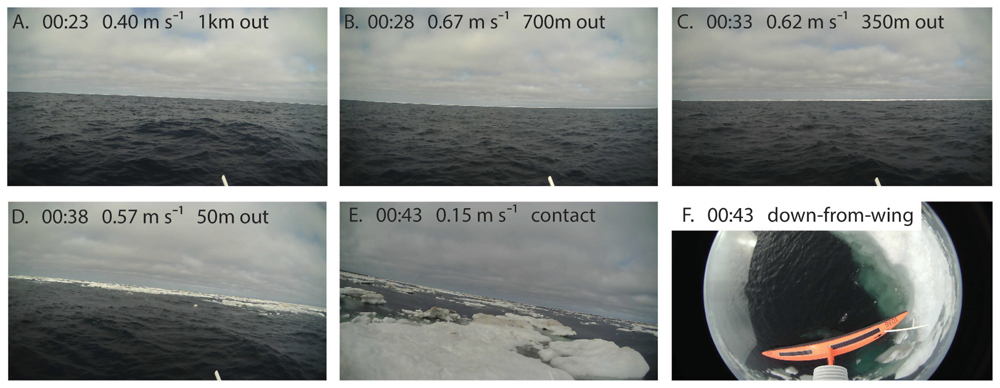
Figure 9. Photos from the camera aboard sd-1036 as it approached the ice band targeted on 18 July 2019. Times in UTC. Distances listed are relative to the vehicle’s northernmost point of travel, at which point it was blocked by ice. Panels (A–E) are looking north, along the vehicle’s northward route. Photo (F) was taken looking down from the top of the vehicle’s wing.
Surface Marine Observations From the Saildrones
Sea ice is known to affect the properties of the seawater around it (e.g., Gallaher et al., 2016; Dewey et al., 2017; Brenner et al., 2020). If the surface marine variables observed in close range of sea ice (say, while ice was visible in the horizontal photos from the vehicles) proved sufficiently distinct from those measured in ice-free water, then they might offer a navigationally useful indicator for the proximity of sea ice. For example, if seawater temperature and salinity falling below a certain level proved to be a sufficiently distinct characteristic of the presence of sea ice, measurements approaching those levels might serve as a warning that vehicle contact with ice was imminent. Examination of the 1-min averaged surface marine observations and navigational metrics collected en route to ice, however, highlights difficulties associated with using surface marine measurements of temperature and salinity for this purpose.
The sd-1036 ice band approach pictured in Figure 9 provides a useful example. The vehicle’s navigational metrics help pinpoint intervals during which the vehicle’s progress was impeded by sea ice. In particular, a drop in vehicle speed from ∼ 0.8 to 0.3 m s–1 was evident between the 39th and 40th minute of 18 July 2019 (Figure 10A; denoted by vertical line). Wind speed remained above ∼ 2.5 m s–1 and the vehicle’s instructions were to maintain course during this time. We thereby infer that ice impeded sd-1036’s northward progress between 00:39 and 00:40 UTC of 18 July 2019. As discussed above, an image confirming that sd-1036 was in contact with sea ice was taken at 00:43. The vehicle remained in the ice from ∼00:40 to 01:08 UTC, after which it made its way back south.
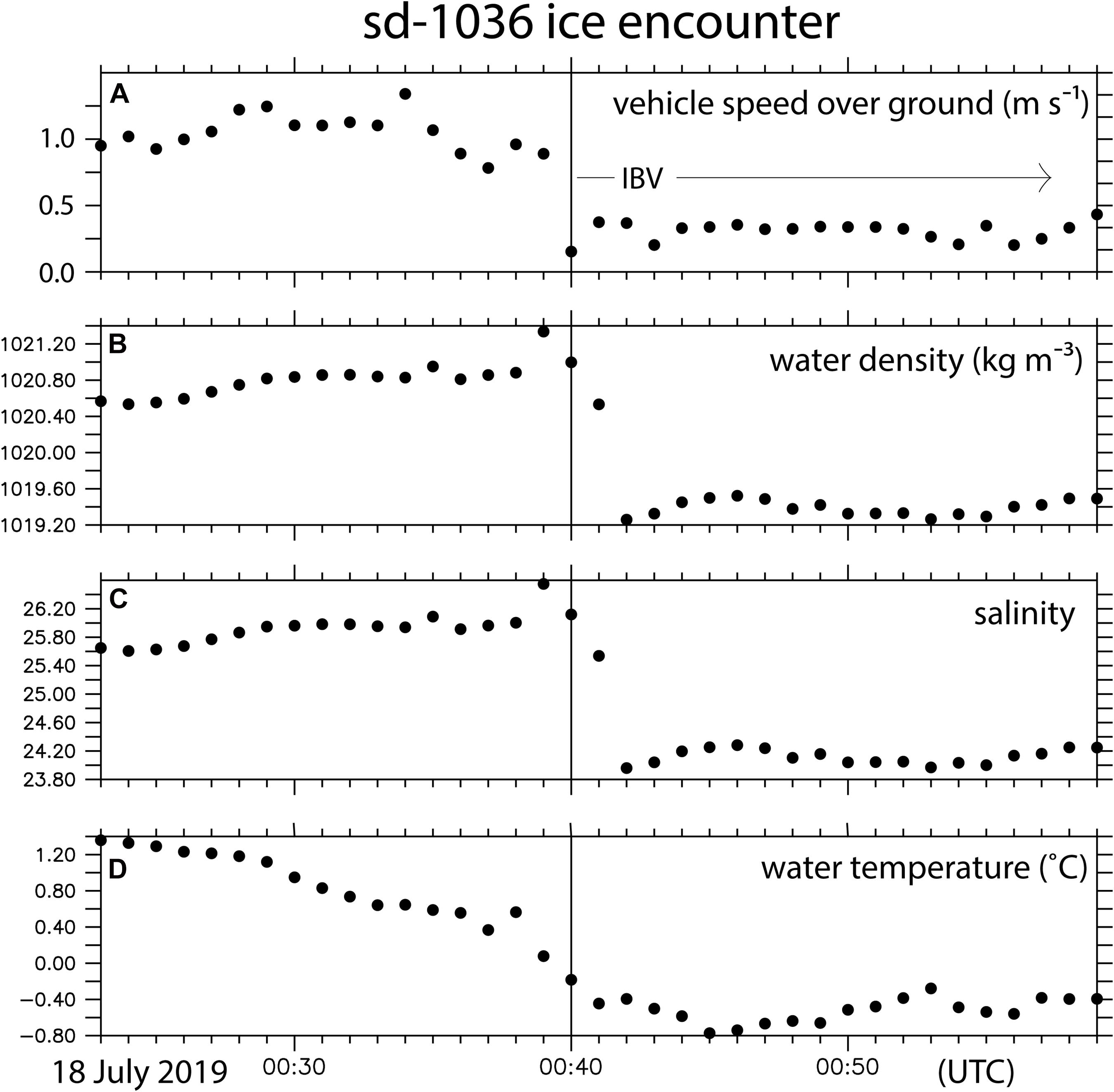
Figure 10. One-minute averaged data just before and after sd-1036 was blocked by sea ice (IBV) on 18 July 2019. (A) The geo-referenced vehicle speed, (B) water density, (C) salinity, and (D) ocean temperature. We infer IBV from the drop in vehicle speed at 00:40 UTC (upper panel; marked with a black vertical line at 00:40 UTC) that sea ice impeded the vehicle’s northward progress sometime between 00:39 and 00:40 UTC. An image confirming that ice was surrounding the vehicle was taken at 00:43 (Figure 9E).
Density, salinity, and temperature values during the ice-band approach are plotted in Figures 10B–D and on a Temperature–Salinity (T–S) plot in Figure 11. At the time of the initial ice contact, at 00:40 UTC, the 1-min averaged measurements for temperature and salinity were −0.18°C and 26.12, which equate to a seawater density near 1021 kg m–3 (Figure 10). A salinity drop of ∼2.2 and temperature drop of ∼0.2°C were observed in the few minutes following 00:40, which lowered the seawater density to ∼1019.5 kg m–3. But this fresher (salinity ∼ 24) and cooler (temperature near −0.5°C) water was observed only after sd-1036 became embedded in the ice band. Even once embedded, temperatures remained above the freezing point (Figure 11). Prior to contact, there was a discernible increase in salinity observed as the vehicle moved closer to the floe (e.g., ∼+0.4 from 00:20 to 00:40). Evidently, at this scale (∼1 km), melting ice is not always located at the low end of an open-water, surface salinity gradient.
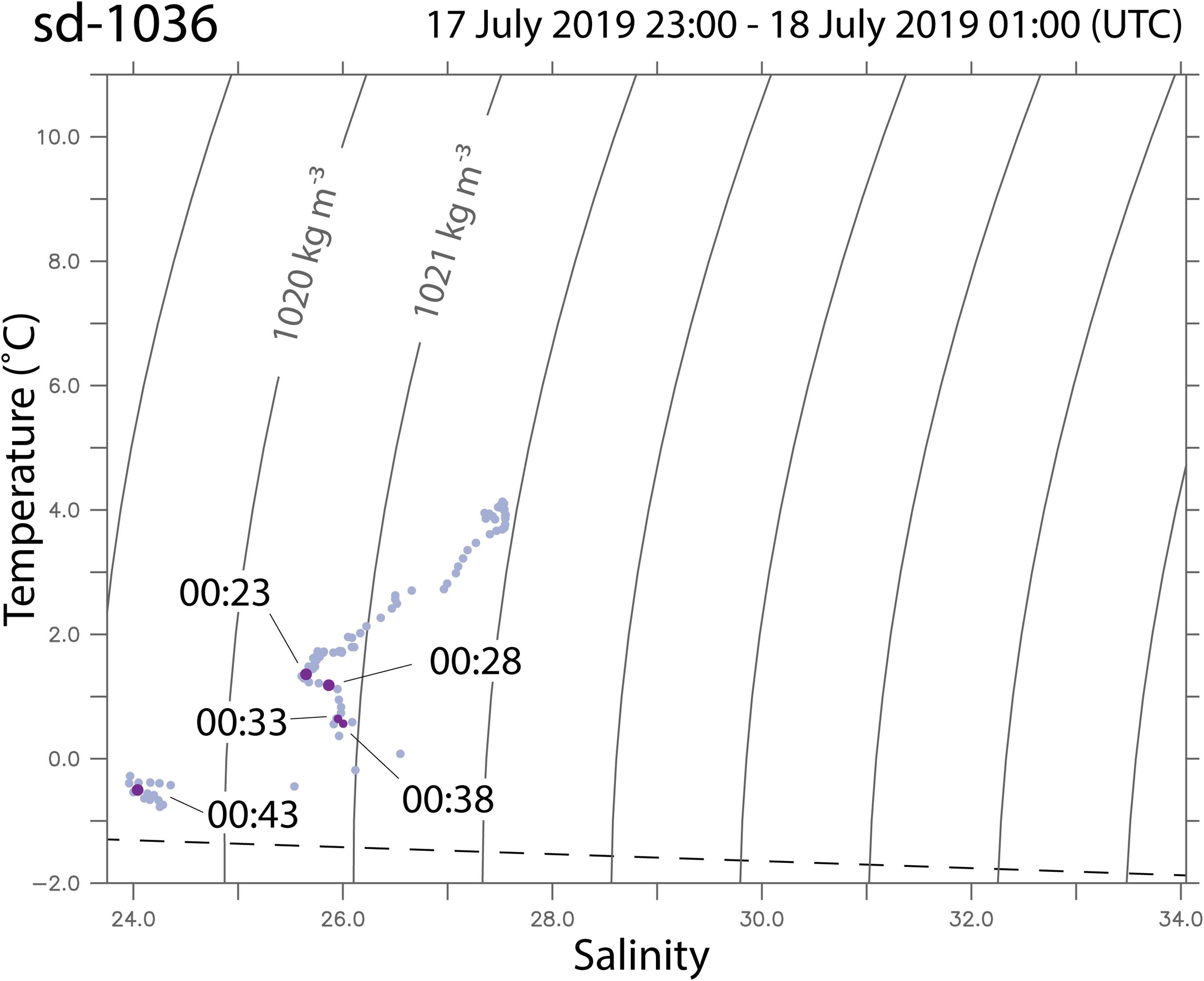
Figure 11. One-minute average temperature and salinity measurements during sd-1036’s initial northward transect into an ice band on 18 July 2019. Density contours every 1 kg m– 3 (solid lines). Seawater freezing temperature calculated based on the equation suggested by Millero and Leung (1976) and used by Fofonoff and Millard (1983) is shown with a dashed line.
Seawater conditions observed just before the ice encounter (i.e., temperatures near 0°C and salinities near 26) were also often observed in ice free water. Figure 12 shows the distribution of 1-min averaged temperatures and salinities collected by sd-1036 during June, July and August, with different symbols differentiating measurements taken while ice was (dots) and was not (open green circles) visible from the vehicle. The low-density (near 1019.5 kg m–3) measurements observed after sd-1036 was embedded in ice on 18 July 2019 are the only ones separated in T–S space from other measurements. The correlation coefficient between sd-1036 temperature (salinity) and the sd-1036 in situ sea-ice time series (equal to 1 when ice was visible, and 0 when ice was not visible in the saildrone images) is −0.37 (−0.26). Based on Bootstrap/Monte Carlo sub-sampling, with replacement, of the respective sd-1036 time series (Efron and Tibshirani, 1991), the temperature correlation with in situ ice is statistically significant at the 99.9% confidence interval and the salinity correlation is significant at the 90% confidence interval. We thus conclude that temperature was more closely related to ice proximity than salinity (c.f. Johnson, 2011) but attempts to use threshold values of seawater temperature and salinity as a proxy for >0% sea-ice concentration in conditions such as were observed by sd-1036 will have a low probability of success.
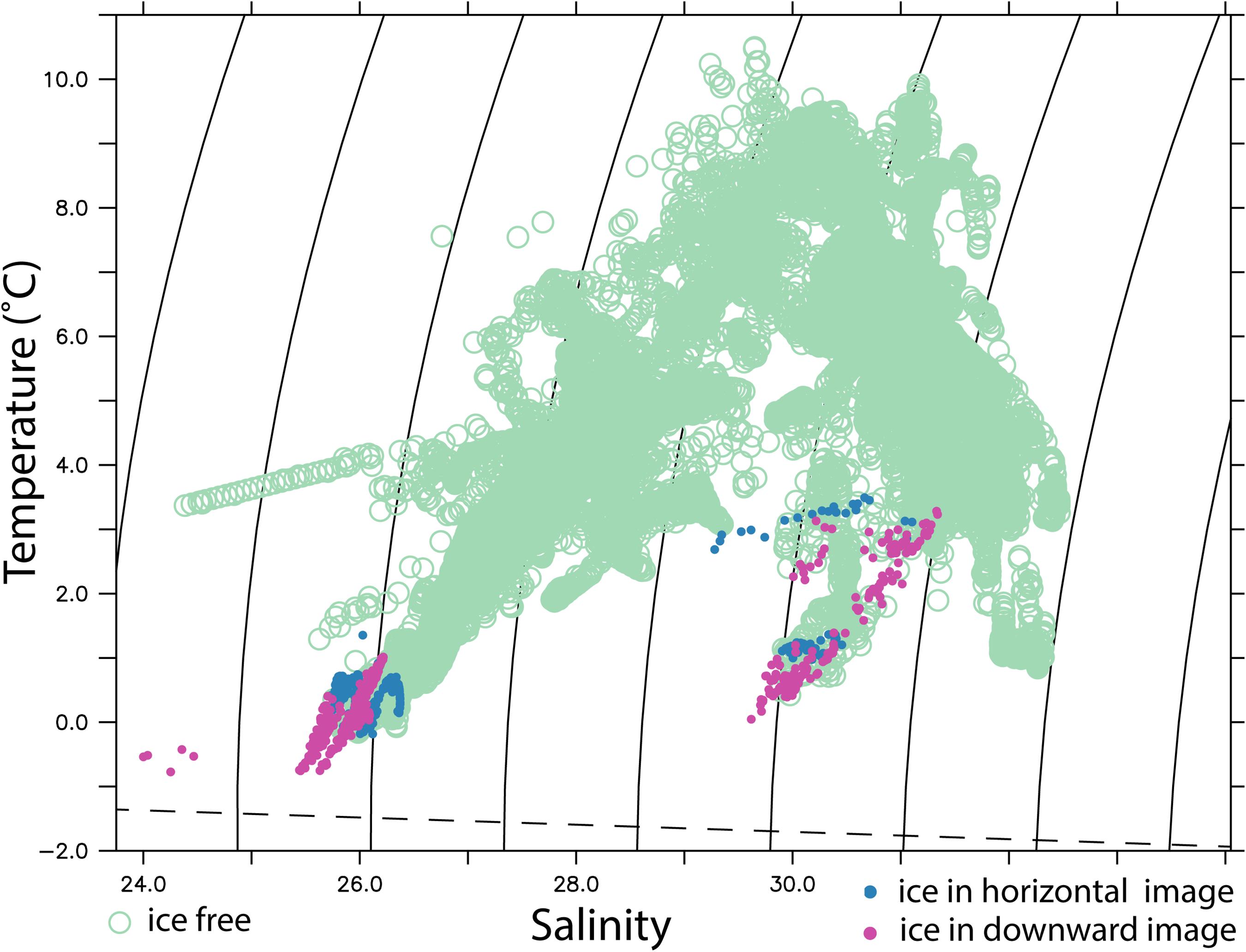
Figure 12. Same as Figure 11 except for seawater temperature and salinity measurements collected by sd-036 during June, July and August of 2019. Light green circles denote times when no ice was visible in the saildrone images; light blue filled dots denote times when ice was visible in the horizontal but not in the downward saildrone photos; magenta dots denote times when ice was visible in the downward-looking saildrone images. Seawater freezing point is shown with a dashed line.
The 18 July 2019 ice encounter described above stood out as a prime candidate for close examination in this context because it was associated with some of the coldest and least saline water observed during the mission. The other ice encounters were also examined for surface marine variable precursors to contact with the ice. Although each encounter differed in detail, when viewed from the perspective of trying to anticipate the transition from open water sailing to probable ice contact, they exhibited broadly similar characteristics. The encounter that led to sd-1035 being embedded in ice for approximately 6 h on 14 June 2019, which was the first such occurrence of the mission, exemplifies these characteristics (Figure 13). In particular, although the salinity and temperature measured while the vehicle was embedded in the ice were substantially lower than those measured when last sailing through open water – in this case temperature dropped by 1.6°C and salinity by 0.7 between 09:10 and 10:10 UTC – most of these changes occurred after the vehicle hit ice at 09:25 UTC. The important point for ice-avoidance navigation is this: The changes observed prior to the point at which the vehicle was impeded by ice – in this case a temperature drop of 0.032°C min–1, or 0.11°C per 100 m based on the 5-min averages centered at 09:10 and 09:23 – were not especially distinct from similar time and space scale changes observed in ice-free water.

Figure 13. As in Figure 9, except for sd-1035’s 14 June 2019 ice encounter. In this case a horizontal photo revealing sparse ice was taken at 09:20 and a downward looking photo confirming ice surrounding the vehicle taken at 09:25 UTC. The drop in vehicle speed over ground between 09:25 and 09:26 (upper-left panel; marked by the IBV-vertical black line in each panel) confirms that the vehicle was impeded then. The blue vertical lines in the near surface water temperature plot (lower left) mark the times of the images shown on the right.
We further examined the temperature and salinity gradients observed during the seven times sd-1036 sailed from open water into the marginal ice zone and was impeded by ice. These spatial gradients appear as temporal tendencies in the saildrone time series. The largest negative tendencies (hereafter, LNTs) observed <3 h before ice contact are listed in Table 1, based on 5 min averages separated by 20 min. The corresponding 1-min averaged temperature and salinity records from these seven ice encounters are also illustrated in Supplementary Figures 5–11. The LNTs preceding four of these seven ice encounters are not very distinct from tendencies seen during periods of ice-free sailing (Figure 14). Specifically, for the 23 June, (2) 6 August and 8 August ice encounters, there were 175–371 other, 3 h-long, ice-free periods that had temporal temperature and salinity LNTs lower than those observed en route to the ice (Table 1). Triggering ice-navigation maneuvers based on temperature and salinity changes in this range (ΔS/Δt = −0.0034 to −0.0082 min–1, ΔT/Δt = −0.0029 to −0.0163°C min–1) would likely introduce unnecessary inefficiency to SIZ sampling strategies because of the apparent abundance of false-positives. Three of these seven ice encounters, however, occurred after traversing stronger gradients than the other 4; the 17 June ice encounter was preceded by a −0.1133°C min–1 temperature (−0.158°C per 100 m) gradient located 4840 m from the ice-blockage point, the 22 June ice encounter by a −0.0371 min–1 (−0.055 per 100 m) salinity gradient observed just before contact with ice, and the 18 July ice encounter by a temperature gradient of −0.0885°C min–1 (−0.119°C per 100 m) and salinity gradient of −0.0686 min–1 (−0.092 per 100 m), each at distance of 1480 m from ice contact (Table 1). Turning the vehicles around based on gradients far from the ice would leave the remaining section of the vehicle route unobserved; thus, the longer of these distances-to-contact (∼1.5 and 5 km) are likely too far for the associated gradients to be used for navigation on their own and still meet our objective of being able to collect observations in close proximity to the ice. The case of navigating based on gradients immediately adjacent to ice presents the opposite issue of needing enough time and space to detect the gradients and turn before contacting the ice; successfully implementing such a system may therefore require refinement. Nonetheless, the stronger gradients associated with these three ice encounters had far fewer (1–19) open-water analogs relative to the other four sd-1036 ice encounters. This suggests that monitoring for negative temperature and salinity tendencies might be useful if a large enough threshold is selected and if supplemented with other ice-detection strategies (see section “Summary and Discussion”).
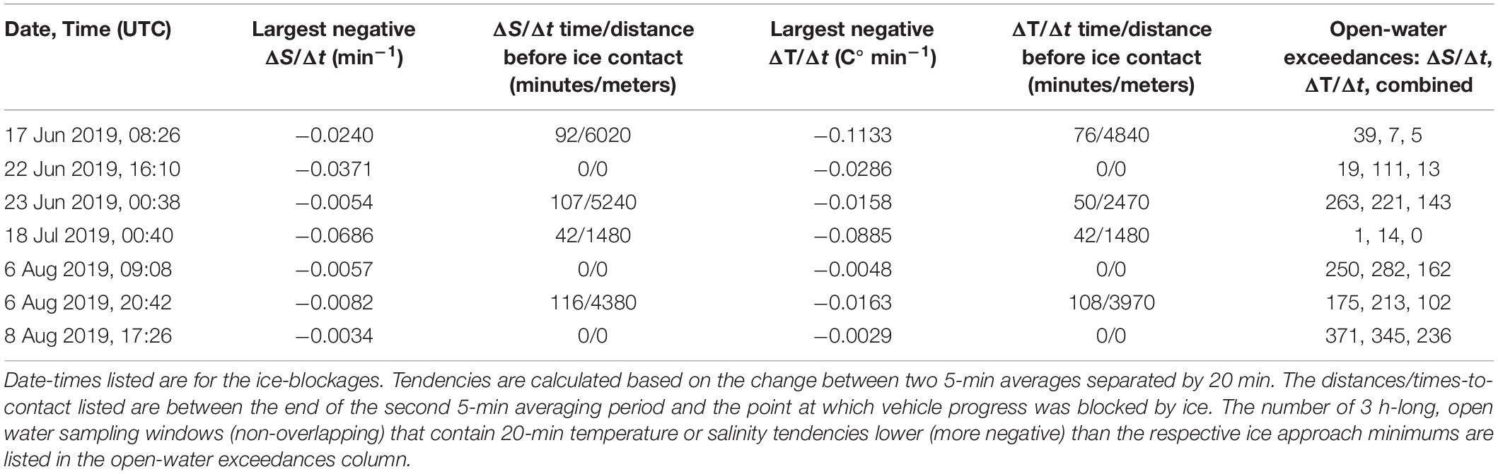
Table 1. Minimum temperature and salinity tendencies observed during seven 3-h-long sd-1036 transects beginning in open water and ending with an IBV (vehicle blocked by sea ice).
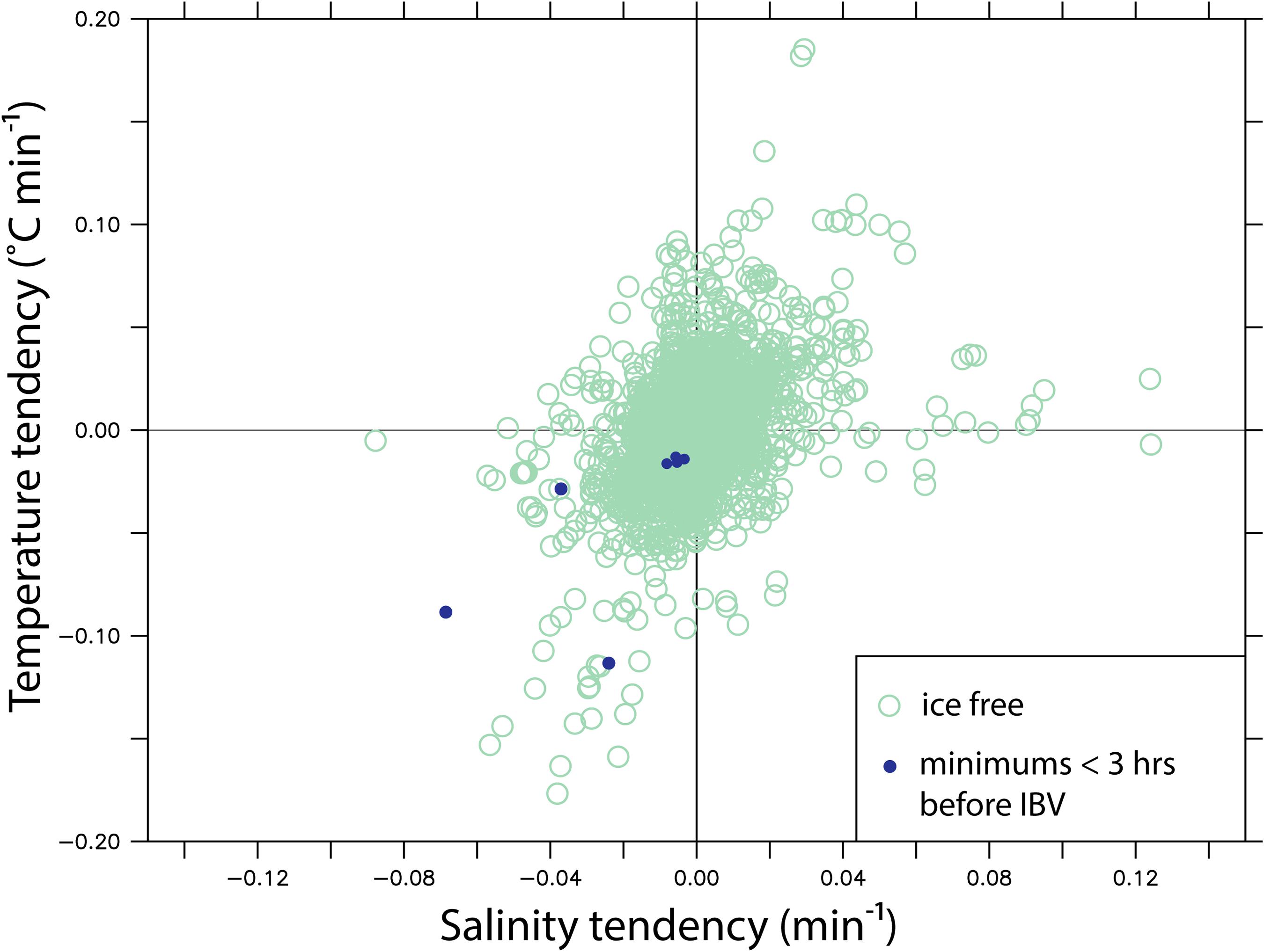
Figure 14. The temperature and salinity tendencies observed while sd-1036 sampled ISSI = 0 conditions (no ice in saildrone images) are plotted with open circles, based on differences between 5 min averages separated by 20 min. The largest negative tendencies observed en route to ice (see Table 1) are plotted with dots.
We also considered other surface marine variables, such as near-surface air temperature and humidity, for use in this context, but failed to find a distinct subset of near-ice values in them (Supplementary Figure 12). The distribution of seawater temperature and salinity values observed while sd-1034 and sd-1035 were embedded in ice and sailing in open water were also examined and found to have character qualitatively similar to the distribution shown Supplementary Figure 12, in that, the subset of in-ice values was indistinct from other values measured in ice-free conditions (the near-1019.5 kg m–3 sd-1036 density values already discussed were the only ones with this distinction). The sd-1034 and sd-1035 temperature and salinity diagrams are therefore not shown for the sake of brevity.
Summary and Discussion
On 15 May 2019 five saildrones were launched from Unalaska (formerly Dutch Harbor), AK, United States with the objective of observing the air-sea interface within the SIZ of the Chukchi and Beaufort Seas. This mission constituted a test of our ability to use saildrones to observe the SIZ with novel instrumentation packages capable of measuring air-sea fluxes of heat, momentum and CO2. These saildrones, however, had not been specifically designed to navigate in close proximity to, or collide with, sea ice.
Remotely controlled navigation near sea ice was a crux of this mission and will remain critical to future attempts to use similar means to provide high quality, in situ observations of surface marine variables in and near the marginal ice zone. Here, we have re-examined the sources of navigational information, based on post-mission tabulation of the sea-ice conditions encountered by the vehicles. Our objectives are to better understand the utility and limitations of this information and to identify opportunities for improving our ability to remotely navigate through the SIZ and near sea ice.
At points in the mission where the vehicles sailed in open water and decisions were being made about where and how to approach marginal ice zones, the EA2 gridded ice-concentration product, pseudo-true color satellite images of the surface and NIC 10% ice concentration contour were initially considered prime candidates for providing regional ice distribution information. However, on most days that the vehicles encountered ice, EA2 estimated zero ice at their location. The chances of seeing ice was not closely linked to EA2 concentration. For example, ice was encountered ∼6% of the time EA2 estimated concentrations of 1–10%, but only ∼4% of the time EA2 estimated >10% concentration. It was also the case that no ice was encountered or photographed by the vehicles on the handful of days in which EA2 predicted the highest ice concentrations (around 20%) at the vehicle locations. These mismatches between the EA2 estimates and in situ conditions encountered by the saildrones made it difficult to reliably use EA2 ice concentration data for SIZ navigation.
We also examined vehicle distances to the daily NIC 10% ice concentration contour on days in which ice was and was not encountered. Our experience with this analysis product largely supports its use as an identifier of ice-free (or nearly so) pathways of navigation over the study region. To put it another way, being on the open water side of the NIC 10% contour proved to be a useful predictor for clear sailing: in only three instances during the mission, specifically on 21 June and 17 August 2019 (sd-1034) and 18 July 2019 (sd-1036) was ice encountered when a vehicle was in waters with discernibly <10% ice concentration according that day’s NIC analysis. And in these three cases the vehicles were close to (within a few to several km from) the NIC 10% contour line. Clear sailing was also encountered, however, most (∼80%) of the time the vehicles were in >10% ice concentration according to NIC. Thus, other information was needed to plan vehicle routes when the navigational objective was not avoiding but sampling close to ice floes.
Satellite-based surface imagery from radiometric measurements in the near-visible range was at times quite useful in this context. On clear-sky days, Sentinel-2 provided relatively high-resolution (10–60 m) images in which ice floes could be distinguished from water with relative ease using imagery that is generally available to the public. MODIS and VIIRS imagery also provided this capability with moderately coarser, but still useful (up to 250 m) horizontal resolution. But this utility was conditional on skies being free enough from clouds to offer clear views of the planetary surface, and this was not the norm during the mission. When cloud cover obscured the optical view of the planetary surface and high-resolution SAR imagery was available to us, it proved very useful, confirming the benefits from investments made in this technology by the European (e.g., Sentinel-1) and Canadian (e.g., Radarsat-2) Space Agencies. The combination of Sentinel-1 and Radarsat-2 coverage, however, suffered from significant time and space gaps in our study region.
The use of USV observations such as near-surface ocean temperature and salinity to help determine proximity to sea ice was examined. Unfortunately, the distributions of these variables exhibited a wide enough range of variability in open water that they often overlapped with characteristics observed just prior to coming into contact with ice floes. This was true for the absolute values of the variables as well as their rates of change in time and space. These overlaps likely preclude this approach from providing, on its own, a reliable indicator that a given vehicle is nearing sea ice. Ice detection, however, was not the main motivation for collecting the surface marine observations. We expect them to be valuable in many other respects. These include providing a basis by which high priority targets for improvements of weather forecast model initializations and predictions can be identified (Zhang et al., submitted) and heat transfer between sea ice and sea water can be estimated.
There might be several reasons for the difficulty of using observed temperature and salinity to detect when USVs are approaching sea ice. If ice floes are drifting toward ice-free water, the strongest temperature and salinity gradients would be very close to their edges facing the ice-free water. Likewise, if surface currents are toward ice bands, they would push relatively warm, saline water against the ice bands and cause the strongest temperature and salinity gradients to lie very close to the ice bands. In addition, sea ice can move quickly (∼2% of the wind speed; Sullivan et al., 2014) leaving behind swaths of melt water that have complex geometrical relationships to the ice before they are mixed to ocean-gyre scales (e.g., Dewey et al., 2017). Other factors, such as the strength of surface wind that dominantly controls surface heat flux, would further complicate distributions of surface temperature relative to sea ice. Distributions of surface temperature and salinity in the SIZ need to be further characterized using the observations from the saildrones deployed in this Arctic mission to better understand both their relationship to sea ice distribution and the time-space sampling density needed to constrain flux estimates over the SIZ.
Based on a review of images taken from the vehicles as they approached waters containing varying concentrations of sea ice, it is not difficult to imagine that – in true real time – they could usefully aid remote navigation near ice bands. For example, they could be used to trigger navigational instructions to the vehicle to preempt unwanted collisions with the ice, or tailor the sampling to mitigate risk to the vehicles if near-ice sampling remained the objective; perhaps by reducing vehicle speed or steering along rather than into a denser ice band. In practice, we found that the delay associated with being able to view the telemetered images (∼ 30–40 min, or 1.8–2.4 km traveling at 1 m s–1) was too long for practical use in this respect. If this transmission time could be greatly reduced, we expect that the images could then play a key role in developing more robust ice zone navigation strategies. However, in the case that this monitoring and navigational decision-making depended upon continued human interaction, the burden this would place on the navigational team during a mission of this length should not be overlooked.
Ideally, artificial intelligence (AI) can be applied to the saildrone images to detect, in real time, sea ice in the distance and either automatically navigate the vehicles to avoid collisions or alert the navigational team. Promising onboard AI navigation strategies have been reported for other USVs previously (e.g., Huntsberger et al., 2011; Carlson et al., 2019; Jin et al., 2020). The power-constraints associated with operating on solar power for months in high-latitudes – and still having power for meteorological and oceanographic sensors – likely preclude many of the specific techniques employed on much shorter missions (e.g., stereo-video cameras, LiDAR) from being very useful for a next generation of Arctic saildrones. However, general advances made recently in image recognition capability (e.g., LeCun et al., 2015) provide a basis for developing this capability. The next generation of saildrones have already been equipped with onboard Artificial Intelligence (AI) navigation for ships (R. Jenkins, pers. comm.). It is unknown if the amount of ice image information collected from this mission is sufficient for a complementary AI application for sea ice. The possibility of applying AI to information from onboard images and in situ observations to develop an automated navigation algorithm for endurance-sailing on solar power in the SIZ should be explored; in this context the in situ saildrone observations (and perhaps satellite information) can be used to add confidence to the ice image detection algorithms. For example, the confidence associated with a possible ice detection in the image algorithm can be downgraded if temperatures are several degrees above the freezing point (SSTs reached 10°C but ice was not seen above 4°C during this mission) or upgraded if temperatures are low and strong negative salinity or temperature gradients are observed.
Although the limitations associated with the ice navigation information available for this mission made it difficult to consistently answer, in a navigationally useful manner, the question of where the ice was in relation to the vehicles without actually running the vehicles into the ice, the mission was completed in October 2019 with some notable successes; saildrones reached latitudes up to 75.49° N and as far east as ∼151°W while traveling over 56,000 km. And although saildrones were not specifically designed to come into contact with ice, they did so on approximately two dozen occasions bracketed by ice-free sailing. Even so, all of the vehicles and the instruments deployed were successfully recovered, although some with damage.
In conclusion, this mission provided understanding toward the potential for USVs to substantially contribute to the development of high-latitude observing systems (e.g., Lee et al., 2017) by providing the capability to accurately monitor surface fluxes of heat, momentum and carbon dioxide throughout the Earth’s SIZ. Improved strategies for remote navigation of the ice zone are needed to accomplish this. Our analysis highlights what appears to be a useful and feasible next step in this process; automated detection of ice from cameras and processors installed on the vehicles that may then trigger navigational maneuvers. The repository of saildrone ice and non-ice images collected on this mission will be key to developing the necessary ice recognition capability. Work is planned to bring this to fruition.
Data Availability Statement
The datasets presented in this study can be found in online repositories. The names of the repository/repositories and accession number(s) can be found below:
https://ferret.pmel.noaa.gov/pmel/erddap/index.html
https://thredds.met.no/thredds/osisaf/osisaf_seaiceconc.html
https://www.natice.noaa.gov/products/daily_products.html
https://worldview.earthdata.nasa.gov/
https://www.sentinel-hub.com/explore/eobrowser/.
Author Contributions
AC co-managed the mission, analysis, design, and writing of this manuscript. CZ was a mission Principal Investigator (PI) and helped design, and write this manuscript. QY co-managed the mission. EC and QY studied a previous year’s ice encounter. EC provided the seminal post-mission tabulation of sea-ice conditions. CMo and PS provided analysis results and aided the writing. CG was a mission PI. JC was a mission PI and helped write this manuscript. NL-S and CMe were instrumental in equipping the saildrones with the observational packages used during this mission. MS, MW, and DH helped organize and write this manuscript. HT led communications with Alaskan communities, helped coordinate the mission’s preparation and progress, and helped write this manuscript. EB and KO’B managed the saildrone data curation, enabled the real-time data feed to the GTS, and helped write this manuscript. All authors contributed to the article and approved the submitted version.
Funding
AC was supported by funding from the NOAA Global Ocean Monitoring and Observation program (FundRef # 100007298). This publication is partially funded by the University of Washington’s Joint Institute for the Study of the Atmosphere and Ocean under NOAA Cooperative Agreement NA15OAR4320063, Contribution No. 2020-1115. MS and CG were funded by the MISST3 Project, NASA grant 80NSSC18K0837. MW gratefully acknowledges support from National Science Foundation Grant 1751363 and the NOAA Arctic Research Program. This is PMEL contribution 5158 and EcoFOCI contribution 0959-RPPO.
Conflict of Interest
The authors declare that the research was conducted in the absence of any commercial or financial relationships that could be construed as a potential conflict of interest.
The reviewer CW declared a shared committee with one of the authors EB at time of review.
Acknowledgments
We thank the Saildrone Inc. team that worked on this mission, including pilots K. Neal, D. Nonweiler, and R. Jenkins who, among other tasks, led the effort to rescue sd-1035, which lost its ability to navigate following the mission’s final ice encounter on 23 Aug 2019. We also thank the members of the Alaskan communities we corresponded with, including those who provided the small boat for sd-1035’s rescue. We thank also Alaska SeaGrant Map Agent Gay Sheffield, NOAA’s Candace Nachman and Amy Holman for continued support in communicating the testing of innovative technologies in the US Arctic. CDR Paul Kunicki helped facilitate communication with the US Coast Guard and researched options for sd-1035’s rescue. We greatly appreciate the assistance from NIC analysists who shared their ice information expertise with us, including Alexandra Darden, William Walter, Chris Readinger, Katie Quinn, Evan Neuworth, Christopher Szorc and Sofia Montalvo. This mission benefited from collaboration and assistance from Kevin Wood, who led aerial reconnaissance of the saildrone positions on 17 July 2019, capturing thermal imaging video of the drones and deploying nearby airborne expendable bathythermographs. This mission benefited from helpful conversation with Luc Rainville and Craig Lee. Ansley Manke contributed FERRET software that calculated distance between saildrones, facilitating close-sail, inter-vehicle sensor comparisons at the beginning and end of the mission. We are also grateful to Stacey Maenner-Jones for remotely controlling the ASVCO2 systems. The saildrone mission was funded by NOAA PMEL Innovative Technology for Arctic Exploration program.
Supplementary Material
The Supplementary Material for this article can be found online at: https://www.frontiersin.org/articles/10.3389/fmars.2021.640697/full#supplementary-material
Footnotes
- ^ saildrone.com
- ^ https://directory.eoportal.org/web/eoportal/satellite-missions/r/radarsat-2
- ^ http://hdl.handle.net/1773/45592
- ^ https://www.sentinel-hub.com/explore/eobrowser/
- ^ https://worldview.earthdata.nasa.gov/
References
Alexander, M. A., Scott, J. D., Friedland, K. D., Mills, K. E., Nye, J. A., Pershing, A. J., et al. (2018). Projected sea surface temperatures over the 21st century: changes in the mean, variability and extremes for large marine ecosystem regions of Northern Oceans. Elem Sci. Anth. 6:9. doi: 10.1525/elementa.191
Banzon, V., Smith, T. M., Steele, M., Huang, B., and Zhang, H. (2020). Improved estimation of proxy sea surface temperature in the Arctic. J. Atmos. Ocean. Technol. 37, 341–349. doi: 10.1175/jtech-d-19-0177.1
Bertoia, C., Manore, M., Andersen, H. S., O’Connors, C., Hansen, K. Q., and Evanego, C. (2004). “‘Chapter 20: synthetic aperture radar for operational ice observation and analysis at the U.S., Canadian and Danish National Ice Centers’,” in Synthetic Aperture Radar: Marine User’s Manual, eds J. R. Apel and C. R. Jackson (Washington, DC: U.S. Dept. of Commerce, National Oceanographic and Atmospheric Administration), 417–442.
Bourassa, M. A., Gille, S. T., Bitz, C., Carlson, D., Cerovecki, I., Clayson, C. A., et al. (2013). High-latitude ocean and sea ice surface fluxes: challenges for climate research. Bull. Am. Meteorol. Soc. 94, 403–423. doi: 10.1175/bams-d-11-00244.1
Brenner, S., Rainville, L., Thomson, J., and Lee, C. (2020). The evolution of a shallow front in the Arctic marginal ice zone. Elem. Sci. Anth. 8:17. doi: 10.1525/elementa.413
Carlson, D. F., Fursterling, A., Versterled, L., Skovby, M., Pedersen, S. S., Melved, C., et al. (2019). An affordable and portable autonomous surface vehicle with obstacle avoidance for coastal ocean monitoring. HardwareX 6:e00059. doi: 10.106/j.ohx.2019.e0059
Cokelet, E. D., Meinig, C., Lawrence-Slavas, N., Stabeno, P. J., Mordy, C. W., Tabisola, H. M., et al. (2015). The Use of Saildrones to Examine Spring Conditions in the Bering Sea. Washington: IEEE.
Danielson, S. L., Ahkinga, O., Ashjian, C., Basyuk, E., Cooper, L. E., Eisner, L., et al. (2020). Manifestation and consequences of warming and altered heat fluxes over the Bering and Chukchi Sea continental shelves. Deep Sea Res. II 177:104781. doi: 10.1016/j.dsr2.2020.104781
Dewey, S. R., Morison, J. H., and Zhang, J. (2017). An Edge-referenced surface fresh layer in the beaufort sea seasonal ice zone. J. Phys. Oceanogr. 47, 1125–1144. doi: 10.1175/JPO-D-16-0158.1
Efron, B., and Tibshirani, R. (1991). Statistical data analysis in the computer age. Science 253, 390–395.
Eriksen, C. C., Osse, T. J., Light, R. D., Wen, T., Lehman, T. W., Sabin, P. L., et al. (2001). Seaglider: a long-range autonomous underwater vehicle for oceanographic research. IEEE J. Ocean. Eng. 26, 424–436. doi: 10.1109/48.972073
Fofonoff, N. P., and Millard, R. C. Jr. (1983). Algorithms for the computation of fundamental properties of seawater. Paper Presented at the UNESCO Technical Papers in Marine Sciences 44. Paris: UNESCO.
Gallaher, S., Stanton, T., Shaw, W., Cole, S. T., Toole, J. M., Wilkinson, J., et al. (2016). Evolution of a Canada Basin ice-ocean boundary layer and mixed layer across a developing thermodynamically forced marginal ice zone. J. Geophys. Res. Oceans 121, 6223–6250. doi: 10.1002/2016JC011778
Gallaher, S. G., Stanton, T. P., Shaw, W. J., Kang, S.-H., Kim, J.-H., and Cho, K.-H. (2017). Field observations and results of a 1-D boundary layer model for developing near-surface temperature maxima in the Western Arctic. Elementa: Sci. Anthropocene 5:11. doi: 10.1525/elementa.195
Grebmeier, J. M., Moore, S. E., Cooper, L. W., and Frey, K. E. (2019). The distributed biological osbervatory: a change detection array in the pacific arctic – an introduction. Deep Sea Res. II 162, 1–7. doi: 10.1016/j.dsr2.2019.05.005
Hui, F., Zhao, T., Li, X., Shokr, M., Heil, P., Zhao, J., et al. (2017). Satellite-based sea ice navigation for Prydz Bay, East Antarctica. Remote Sens. 9:518. doi: 10.3390/rs9060518
Huntsberger, T., Aghazarian, H., Howard, A., and Trotz, D. C. (2011). Stereo vision-based navigation for autonomous surface vessels. J. Field Robot. 28, 3–18. doi: 10.1002/rob.20380
IACS (2016). International Association of Classification Societies, Unified Requirements for Polar Class Ships (UR-I). Rev. 2. Available online at: https://www.iacs.org.uk/download/1803 (accessed March 2021).
Ice Navigation in Canadian Waters (2012). Ottowa: Icebreaking Program, Maritime Services Canadian Coast Guard Fisheries and Oceans Canada. Ottowa: Ice Navigation in Canadian Waters, 81–115.
Jayne, S., and Bogue, N. (2017). Air-deployable profiling floats. Oceanography 30, 29–31. doi: 10.5670/oceanog.2017.214
Jin, J., Zhang, J., Liu, D., Shi, J., Wang, D., and Li, F. (2020). Vision-based target tracking for unmanned surface vehicle considering its motion features. IEEE Access 8, 132655–132664. doi: 10.1109/ACCESS.2020.3010327
Johnson, W. (2011). Correlation and explaining variance: to square or not to square? Intelligence 39, 249–254. doi: 10.1016/j.intell.2011.07.001
Karvonen, J. (2017). Baltic sea ice concentration estimation using SENTINEL-1 SAR and AMSR2 microwave radiometer data. IEEE Trans. Geosci. Remote Sens. 55, 2871–2883. doi: 10.1109/TGRS.2017.2655567
Kashiwase, H., Ohshima, K. I., Nihashi, S., and Eicken, H. (2017). Evidence for ice-ocean albedo feedback in the Arctic Ocean shifting to a seasonal ice zone. Sci. Rep. 7:8170. doi: 10.1038/s41598-017-08467-z
König, M., Hieronymi, M., and Oppelt, N. (2019). Application of Sentinel-2 MSI in arctic research: evaluating the performance of atmospheric correction approaches over arctic sea ice. Front. Earth Sci. 7:22. doi: 10.3389/feart.2019.00022
Lavelle, J., Tonboe, R., Pfeiffer, R.-H., and Howe, E. (2016). Validation Report for the OSI SAF AMSR-2 Sea Ice Concentration, Product OSI-408. Version 1.1. Available online at: http://saf.met.no/docs/osisaf_cdop2_ss2_valrep_amsr2-ice-conc_v1p1.pdf (accessed March, 2021).
LeCun, Y., Bengio, Y., and Hinton, G. (2015). Deep learning. Nature 521, 436–444. doi: 10.1038/nature14539
Lee, C. M., Sylvia, C., Martin, D., James, M., Ruth, M., and Tom, P. (2016). Stratified Ocean Dynamics in the Arctic: Science and Experiment Plan. Seattle, WC: Applied Physical Laboratory, University of Washington. Technical Report APL-UW TR 1601.
Lee, C. M., Thomson, J., and the Marginal Ice Zone and Arctic Sea State Teams (2017). An autonomous approach to observing the seasonal ice zone in the western Arctic. Oceanography 30, 56–68. doi: 10.5670/oceanog.2017.222
Levine, R., De Robertis, A., Grunbaum, D., Woodgate, R., Mordy, C., Mueter, F. J., et al. (2020). Repeat autonomous vehicle surveys indicate that age-0 gadid fishes are largely retained over the Chukchi Sea shelf in summer 2018. Limnol. Oceanogr. [Epub ahead of print].
Li, M., Pickart, R. S., Spall, M. A., Weingartner, T. J., Lin, P., Moore, G. W. K., et al. (2019). Circulation of the Chukchi Sea shelfbreak and slope from moored timeseries. Prog. Oceanogr. 172, 14–33. doi: 10.1016/j.pocean.2019.01.002
Liu, Z., Schweiger, A., and Lindsay, R. (2015). Observations and modeling of atmospheric profiles in the arctic seasonal ice zone. Monthly Weather Rev. 143, 39–53. doi: 10.1175/MWR-D-14-00118.1
Lu, K., Danielson, S., Hedstrom, K., and Weingarner, T. (2020). Assessing the role of oceanic heat fluxes on ice ablation of the central Chukchi Sea Shelf. Prog. Oceanogr. 184:102313. doi: 10.1016/j.pocean.2020.102313
Markus, T., and Dokken, S. T. (2002). Evaluation of late summer passive microwave arctic sea ice retrievals. IEEE Trans. Geosci. Remote Sens. 40, 348–356. doi: 10.1109/36.992795
Meinig, C., Burger, E. F., Cohen, N., Cokelet, E. D., Cronin, M. F., Cross, J. N., et al. (2019). Public–private partnerships to advance regional ocean-observing capabilities: a saildrone and NOAA-PMEL case study and future considerations to expand to global scale observing. Front. Mar. Sci. 6:448. doi: 10.3389/fmars.2019.00448
Meinig, C., Jenkins, R., Lawrence-Slavas, N., and Tabisola, H. (2015). “The use of Saildrones to examine spring conditions in the Bering Sea: vehicle specification and mission performance,” in Proceedings of the Oceans 2015 MTS/IEEE, Marine Technology Society and Institute of Electrical and Electronics Engineers, Washington, DC.
Millero, F. J., and Leung, W. H. (1976). The thermodynamics of seawater at one atmosphere. Am. J. Sci. 276, 1035–1077. doi: 10.2475/ajs.276.9.1035
Mordy, C. W., Cokelet, E. D., DeRobertis, A., Jenkins, R., Kuhn, C. E., Lawrence-Slavas, N., et al. (2017). Advances in ecosystem research: saildrone surveys of oceanography, fish, and marine mammals in the Bering Sea. Oceanography 30, 113–115. doi: 10.5670/oceanog.2017.230
Nagler, T., Rott, H., Hetzenecker, M., Wuite, J., and Potin, P. (2015). The sentinel-1 mission: new opportunities for ice sheet observations. Remote Sens. 7, 9371–9389. doi: 10.3390/rs70709371
Ouyang, Z., Qi, D., Chen, L., Takahashi, T., Zhong, W., DeGrandpre, M. D., et al. (2020). Sea-ice loss amplifies summertime decadal CO2 increase in the western Arctic Ocean. Nat. Clim. Chang. 10, 678–684. doi: 10.1038/s41558-020-0784-2
Polashenski, C., Perovich, D., Richter-Menge, J., and Elder, B. (2011). Seasonal ice mass-balance buoys: adapting tools to the changing Arctic. Ann. Glaciol. 52, 18–26. doi: 10.3189/172756411795931516
Qi, D., Chen, B., Chen, L., Lin, H., Gao, Z., Sun, H., et al. (2020). Coastal acidification induced by biogeochemical processes driven by sea-ice melt in the western Arctic ocean. Polar Sci. 23:100504. doi: 10.1016/j.polar.2020.100504
Rainville, L., Wilkinson, J., Durley, M. E., Harper, S., DiLeo, J., Doble, M., et al. (2020). Improving situational awareness in the Arctic Ocean. Front. Mar. Sci. 7:581139. doi: 10.3389/fmars.2020.581139
Sabine, C., Sutton, A., McCabe, K., Noah, L. S., Simone, A., Richard, F., et al. (2020). Evaluation of a new carbon dioxide system for autonomous surface vehicles. J. Atmos. Ocean. Tech. 37, 1305–1317. doi: 10.1175/jtech-d-20-0010.1
Scheuchl, B., Flett, D., Caves, R., and Cumming, I. (2004). Potential of Radarsat-2 data for operational sea ice monitoring. Can. J. Remote Sens. 30, 448–461. doi: 10.5589/m04-011
Serreze, M. C., and Francis, J. A. (2006). The arctic amplification debate. Clim. Change 76, 241–264. doi: 10.1007/s10584-005-9017-y
Smith, L. C., and Stephensen, S. R. (2013). New Trans-Arctic shipping routes navigable by midcentury. Proc. Nat. Adac. Sci. U.S.A. 110, E1191–E1195. doi: 10.1073/pnas.1214212110
Stabeno, P. J. (2019). The Eastern Bering Sea: declining ice, warming seas, and a changing ecosystem, in State of the Climate in 2018. Bull. Am. Meteorol. Soc. 100, S148–S149. doi: 10.1175/2019BAMSStateoftheClimate.1
Stabeno, P. J., and Bell, S. W. (2019). Extreme conditions in the Bering Sea (2017-2018): record breaking low sea-ice extent. Geophys. Res. Lett. 46, 8952–8959. doi: 10.1029/2019GL083816
Steele, M., and Ermold, W. (2015). Loitering of the retreating sea ice edge in the Arctic Seas. J. Geophys. Res. Oceans 120, 7699–7721. doi: 10.1002/2015JC011182
Stoddard, M. A., Etienne, L., Fournier, M., Pelot, R., and Beveridge, L. (2016). Making sense of arctic maritime traffic using the polar operational limits assessment risk indexing system (POLARIS). IOP Conf. Ser. Earth Environ. Sci. 34:e012034.
Sullivan, M. E., Kachel, N. B., Mordy, C. W., Salo, S. A., and Stabeno, P. J. (2014). Sea ice and water column structure on the eastern Bering sea shelf. Deep Sea Res. II 109, 39–56. doi: 10.1016/j.dsr2.2014.05.009
Sutton, A. J., Sabine, C. L., Maenner-Jones, S., Lawrence-Slavas, N., Meinig, C., Feely, R. A., et al. (2014). A high-frequency atmospheric and seawater pCO2 data set from 14 open-ocean sites using a moored autonomous system. Earth Syst. Sci. 6, 353–366. doi: 10.5194/essd-6-353-2014
Terhaar, J., Kwiatkowski, L., and Bopp, L. (2020). Emergent constraint on Arctic Ocean acidification in the twenty-first century. Nature 582, 379–383. doi: 10.1038/s41586-020-2360-3
Thomson, J. (2012). Wave breaking dissipation observed with “SWIFT” drifters. J. Atmos. Ocean. Technol. 29, 1866-1882. doi: 10.1175/JTECH-D-12-00018.1
Timmermans, M.-L., Proshutinsky, A., Golubeva, E., Jackson, J. M., Krishfield, R., McCall, M., et al. (2014). Mechanisms of pacific summer water variability in the arctic’s Central Canada Basin. J. Geophys. Res. 119, 7523-7548. doi: 10.1002/2014JC010273
Transport Canada (2018). Arctic Ice Regime Shipping System (AIRSS) Standard. TP 12259. Canada: Transport Canada.
U.S. National Ice Center (2020). U.S. National Ice Center Daily Marginal Ice Zone Products, Version 1. Overlay Shapefile and User Guide. Boulder, CA: NSIDC: National Snow and Ice Data Center.
Walsh, J. E. (2014). Intensified warming of the Arctic: causes and impacts on middle latitudes. Glob. Planet. Change 117, 52–63. doi: 10.1016/j.gloplacha.2014.03.003
Wang, M., and Overland, J. E. (2009). A sea ice free summer Arctic within 30 years? Geophys. Res. Lett. 36:L07502. doi: 10.1029/2009GL037820
Wang, M., and Overland, J. E. (2012). A sea ice free summer Arctic within 30 years – an update from CMIP5 models. Geophys. Res. Lett. 39:L18501. doi: 10.1029/2012GL052868
Wang, M., Yang, Q., Overland, J. E., and Stabeno, P. J. (2018). Sea-ice cover timing in the Pacific Arctic: the present and projections to mid-century by selected CMIP5 models. Deep Sea Res. II 152, 22–34. doi: 10.1016/j.dsr2.2017.11.017
Wood, K., Overland, J. E., Salo, S. A., Bond, N. A., Williams, W. J., and Dong, X. (2013). Is there a “new normal” climate in the Beafort Sea? Polar Res. 32:19552. doi: 10.3402/polar.v32i0.19552
Zakhvatkina, N., Korosov, A., Muckenhuber, S., Sandven, S., and Babiker, M. (2017). Operational algorithm for ice-water classification on dula-polarized RADARSAT-2 images. Cryosphere 11, 33–46. doi: 10.5194/tc-11-33-2017
Zakhvatkina, N., Smirnov, V., and Bychkova, I. (2019). Satellite SAR data-based sea ice classification: an overview. Geosciences 9:152. doi: 10.3390/geosciences9040152
Keywords: Arctic sea ice, saildrone, USVs, satellite sea-ice concentration, remote navigation, air-sea fluxes, surface marine observations, ice navigation
Citation: Chiodi AM, Zhang C, Cokelet ED, Yang Q, Mordy CW, Gentemann CL, Cross JN, Lawrence-Slavas N, Meinig C, Steele M, Harrison DE, Stabeno PJ, Tabisola HM, Zhang D, Burger EF, O’Brien KM and Wang M (2021) Exploring the Pacific Arctic Seasonal Ice Zone With Saildrone USVs. Front. Mar. Sci. 8:640690. doi: 10.3389/fmars.2021.640697
Received: 11 December 2020; Accepted: 12 April 2021;
Published: 03 May 2021.
Edited by:
Gilles Reverdin, Centre National de la Recherche Scientifique (CNRS), FranceReviewed by:
Christoph Waldmann, University of Bremen, GermanyAlexandre Supply, Laboratoire de physique des océans et de télédétection par satellite (LOPS), France
Copyright © 2021 Chiodi, Zhang, Cokelet, Yang, Mordy, Gentemann, Cross, Lawrence-Slavas, Meinig, Steele, Harrison, Stabeno, Tabisola, Zhang, Burger, O’Brien and Wang. This is an open-access article distributed under the terms of the Creative Commons Attribution License (CC BY). The use, distribution or reproduction in other forums is permitted, provided the original author(s) and the copyright owner(s) are credited and that the original publication in this journal is cited, in accordance with accepted academic practice. No use, distribution or reproduction is permitted which does not comply with these terms.
*Correspondence: Andrew M. Chiodi, andy.chiodi@noaa.gov
†Present address: Qiong Yang, The Climate Corporation, Seattle, WA, United States